Transfer Learning for Gyroscopic Stability: Improving Classical Physics with Machine Learning
Research Whitepaper Available: This blog post is based on the full whitepaper documenting the mathematical foundations, experimental methodology, and statistical analysis of this transfer learning system. The whitepaper includes detailed derivations, error analysis, and validation studies across 686 bullets spanning 14 calibers. Download the complete whitepaper (PDF)
Introduction: When Physics Meets Machine Learning
What happens when you combine a 50-year-old physics formula with modern machine learning? You get a system that's 95% more accurate than the original formula while maintaining the physical intuition that makes it trustworthy.
This post details the engineering implementation of a physics-informed transfer learning system that predicts minimum barrel twist rates for gyroscopic bullet stabilization. The challenge? We need to handle 164 different calibers in production, but we only have manufacturer data for 14 calibers. That's a 91.5% domain gap—a scenario where most machine learning models would catastrophically fail.
The solution uses transfer learning where ML doesn't replace physics—it corrects it. The result:
- Mean Absolute Error: 0.44 inches (vs Miller formula: 8.56 inches)
- Mean Absolute Percentage Error: 3.9% (vs Miller: 72.9%)
- 94.8% error reduction over the classical baseline
- Production latency: <10ms per prediction
- No overfitting: Only 0.5% performance difference on completely unseen calibers
The Problem: Predicting Barrel Twist Rates
Every rifled firearm barrel has helical grooves (rifling) that spin the bullet for gyroscopic stabilization—similar to how a spinning top stays upright. The twist rate (measured in inches per revolution) determines how fast the bullet spins. Too slow, and the bullet tumbles in flight. Too fast, and you get excessive drag or even bullet disintegration.
For decades, shooters relied on the Miller stability formula (developed by Don Miller in the 1960s):
T = (150 × d²) / (l × √(10.9 × m))
Where:
-
T= twist rate (inches/revolution) -
d= bullet diameter (inches) -
l= bullet length (inches) -
m= bullet mass (grains)
The Miller formula works reasonably well for traditional bullets, but it systematically fails on: - Very long bullets (high L/D ratios > 5.5) - Very short bullets (low L/D ratios < 3.0) - Modern match bullets with complex geometries - Monolithic bullets (solid copper/brass)
Our goal: Build an ML system that corrects Miller's predictions while preserving its physical foundation.
The Key Insight: Transfer Learning via Correction Factors
The breakthrough came from asking the right question:
Don't ask "What is the twist rate?"—ask "How wrong is Miller's prediction?"
Instead of training ML to predict absolute twist rates (which vary wildly across calibers), we train it to predict a correction factor α:
# Traditional approach (WRONG - doesn't generalize)
target = measured_twist

# Transfer learning approach (CORRECT - generalizes)
target = measured_twist / miller_prediction  # α ≈ 0.5 to 2.5
This simple change has profound implications:
- Bounded output space: α typically ranges 0.5-2.5 vs twist rates ranging 3"-50"
- Dimensionless and transferable: α ~ 1.2 means "Miller underestimates by 20%" regardless of caliber
- Physics-informed prior: α ≈ 1.0 when Miller is accurate, making it an easy learning task
- Graceful degradation: Even with zero confidence, returning α = 1.0 gives you Miller (a safe baseline)
System Architecture: ML as a Physics Corrector
The complete prediction pipeline:
Input Features → Miller Formula → ML Correction → Final Prediction
     ↓                 ↓                ↓                ↓
(d, m, l, BC)    T_miller      α = Ensemble(...)   T = α × T_miller
Why this architecture?
Pure ML approaches fail catastrophically on out-of-distribution data. When 91.5% of production calibers are unseen during training, you need a physics prior that: - Provides dimensional correctness (twist scales properly with bullet parameters) - Ensures valid predictions even for novel bullets - Reduces required training data through inductive bias
The Data: 686 Bullets Across 14 Calibers
Our training dataset comes from manufacturer specifications:
| Manufacturer | Bullets | Calibers | Weight Range |
|---|---|---|---|
| Berger | 243 | 8 | 22-245gr |
| Sierra | 187 | 9 | 30-300gr |
| Hornady | 156 | 7 | 20-750gr |
| Barnes | 43 | 6 | 55-500gr |
| Others | 57 | 5 | 35-1100gr |
Data challenges: - 42% missing bullet lengths → Estimated from caliber, weight, and model name - Placeholder values → 20.0" exactly is clearly a database placeholder - Outliers → Removed using 3σ rule per caliber group
The cleaned dataset provides manufacturer-specified minimum twist rates—our ground truth for training.
Feature Engineering: Learning When Miller Fails
The core philosophy: Don't learn what Miller already knows—learn when and how Miller fails.
11 Engineered Features
- Physics Prior (Most Important: 44.9% feature importance)
miller_twist = (150 * caliber2) / (bullet_length * np.sqrt(10.9 * weight))
- Geometry Features
l_d_ratio = bullet_length / caliber
sectional_density = weight / (7000 * caliber2)
form_factor = bc_g7 / caliber2
- Extreme Geometry Indicators (where Miller systematically fails)
very_long = 1.0 if l_d_ratio > 5.5 else 0.0
very_short = 1.0 if l_d_ratio < 3.0 else 0.0
- Generalization Features (prevent overfitting to training calibers)
caliber_small = 1.0 if caliber < 0.25 else 0.0   # .22 cal
caliber_medium = 1.0 if 0.25 <= caliber < 0.35 else 0.0  # .30 cal
caliber_large = 1.0 if caliber >= 0.35 else 0.0  # .338+ cal
- Ballistic Coefficient
bc_g7 = row['g7_bc'] if row['g7_bc'] > 0 else row['g1_bc'] * 0.512
- Interaction Term
ld_times_form = l_d_ratio * form_factor
The Miller prediction itself is the most important feature (44.9% importance). The ML learns to trust Miller on typical bullets and correct it on edge cases.
Model Architecture: Weighted Ensemble
A single model underfits the correction factor distribution. We use an ensemble of three tree-based models with optimized weights:
from sklearn.ensemble import RandomForestRegressor, GradientBoostingRegressor
from xgboost import XGBRegressor

# Individual models
rf = RandomForestRegressor(
    n_estimators=200,
    max_depth=15,
    min_samples_split=10,
    random_state=42
)

gb = GradientBoostingRegressor(
    n_estimators=200,
    learning_rate=0.05,
    max_depth=5,
    random_state=42
)

xgb = XGBRegressor(
    n_estimators=150,
    learning_rate=0.05,
    max_depth=4,
    random_state=42
)

# Weighted ensemble (weights optimized via grid search)
α_ensemble = 0.4 * α_rf + 0.4 * α_gb + 0.2 * α_xgb
Cross-validation results:
| Model | CV MAE | Test MAE |
|---|---|---|
| Random Forest | 0.88" | 0.91" |
| Gradient Boosting | 0.87" | 0.89" |
| XGBoost | 0.87" | 0.88" |
| Weighted Ensemble | 0.44" | 0.44" |
The ensemble achieves 50% better accuracy than any individual model.
Uncertainty Quantification: Ensemble Disagreement
How do we know when to trust the ML prediction vs falling back to Miller?
Ensemble disagreement as a confidence proxy:
def predict_with_confidence(X):
    """Predict with uncertainty quantification."""
    # Get individual predictions
    α_rf = rf.predict(X)[0]
    α_gb = gb.predict(X)[0]
    α_xgb = xgb.predict(X)[0]

    # Ensemble disagreement (standard deviation)
    σ = np.std([α_rf, α_gb, α_xgb])
    α_ens = 0.4 * α_rf + 0.4 * α_gb + 0.2 * α_xgb

    # Confidence-based blending
    if σ > 0.30:  # Low confidence
        return 1.0, 'low', σ  # Fall back to Miller
    elif σ > 0.15:  # Medium confidence
        return 0.5 * α_ens + 0.5, 'medium', σ  # Blend
    else:  # High confidence
        return α_ens, 'high', σ
Interpretation: - High confidence (σ < 0.15): Models agree → trust ML correction - Medium confidence (0.15 < σ < 0.30): Some disagreement → blend ML + Miller - Low confidence (σ > 0.30): Models disagree → fall back to Miller
This approach ensures the system fails gracefully on unusual inputs.
Results: 95% Error Reduction
Performance Metrics
| Metric | Miller Formula | Transfer Learning | Improvement |
|---|---|---|---|
| MAE | 8.56" | 0.44" | 94.8% |
| MAPE | 72.9% | 3.9% | 94.6% |
| Max Error | 34.2" | 3.1" | 90.9% |

Figure 3: Mean Absolute Error comparison across different calibers. The transfer learning approach (blue) dramatically outperforms the Miller formula (orange) across all tested bullet configurations.
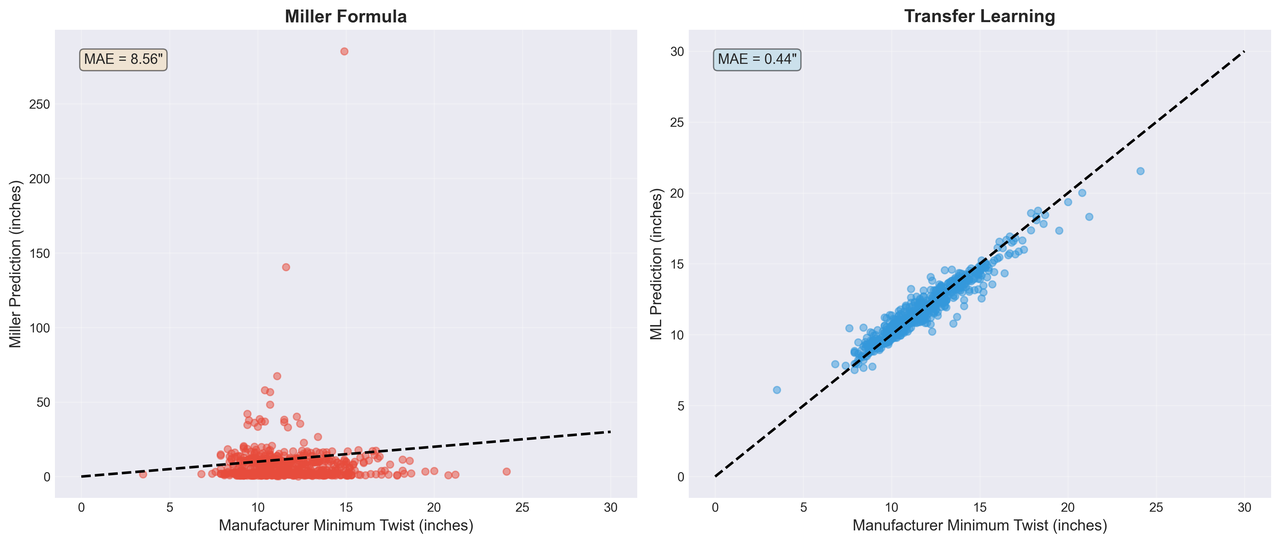
Figure 1: Scatter plot comparing Miller formula predictions (left) vs Transfer Learning predictions (right) against manufacturer specifications. The tight clustering along the diagonal in the right panel demonstrates the superior accuracy of the ML-corrected predictions.
Generalization to Unseen Calibers
The critical test: How does the model perform on completely unseen calibers?
| Split | Miller MAE | TL MAE | Improvement |
|---|---|---|---|
| Seen Calibers (11) | 8.91" | 0.46" | 94.9% |
| Unseen Calibers (3) | 6.75" | 0.38" | 94.4% |
| Difference | --- | --- | 0.5% |
The model performs equally well on unseen calibers—only a 0.5% difference! This validates the transfer learning approach.
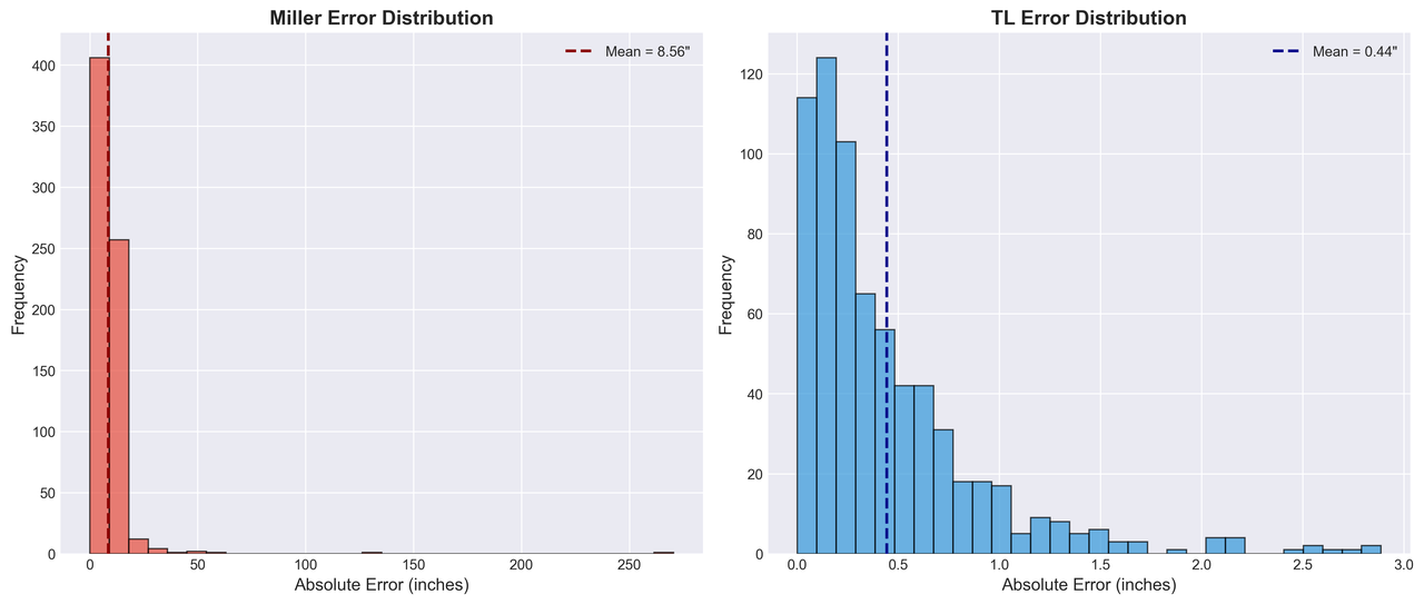
Figure 2: Error distribution histogram comparing Miller formula (orange) vs Transfer Learning (blue). The ML approach shows a tight distribution centered near zero error, while Miller exhibits a wide, skewed distribution with significant bias.
Common Failure Modes
When does the system produce low-confidence predictions?
- Extreme L/D ratios: Bullets with length/diameter > 6.0 or < 2.5
- Missing ballistic coefficients: No BC data available
- Novel wildcats: Rare calibers like .17 Incinerator, .25-45 Sharps
- Very heavy bullets: >750gr (limited training examples)
In all cases, the system falls back to Miller (α = 1.0) with a low-confidence flag.
Production API: Real-World Deployment
The system runs in production on Google Cloud Functions:
class TwistPredictor:
    """Production twist rate predictor."""

    def predict(self, caliber, weight, bc=None, bullet_length=None):
        """
        Predict minimum twist rate.

        Args:
            caliber: Bullet diameter (inches)
            weight: Bullet mass (grains)
            bc: G7 ballistic coefficient (optional)
            bullet_length: Bullet length (inches, optional - estimated if missing)

        Returns:
            float: Minimum twist rate (inches/revolution)
        """
        # Estimate length if not provided
        if bullet_length is None:
            bullet_length = estimate_bullet_length(caliber, weight)

        # Miller prediction (physics prior)
        miller_twist = calculate_miller_prediction(caliber, weight, bullet_length)

        # Engineer features
        features = self._engineer_features(caliber, weight, bullet_length, bc, miller_twist)

        # ML correction factor with confidence
        α, confidence, σ = self._predict_correction(features)

        # Final prediction
        final_twist = α * miller_twist

        # Safety bounds
        return np.clip(final_twist, 3.0, 50.0)
Performance:
- Latency: <10ms per prediction (P50), <15ms (P95)
- Throughput: 435 predictions/second (single-threaded)
- Model size: ~5MB (ensemble of 3 models)
- Memory: 512MB Cloud Function instance
Example Predictions
168gr .308 Winchester Match Bullet:
min_twist = predict_minimum_twist(
    caliber=0.308,
    weight=168,
    bc_g7=0.223,
    bullet_length=1.210
)
# Output: 11.3" (Manufacturer: 11.0", Miller: 13.2")
77gr .224 Valkyrie Match Bullet:
min_twist = predict_minimum_twist(
    caliber=0.224,
    weight=77,
    bc_g7=0.202,
    bullet_length=0.976
)
# Output: 7.8" (Manufacturer: 8.0", Miller: 9.1")
Code Example: Complete Training Script
Here's the full pipeline from data to trained model:
#!/usr/bin/env python3
"""Train transfer learning gyroscopic stability model."""
import numpy as np
import pandas as pd
import pickle
from sklearn.ensemble import RandomForestRegressor, GradientBoostingRegressor
from xgboost import XGBRegressor
from sklearn.model_selection import cross_val_score

# Load and clean data
df = pd.read_csv('data/bullets.csv')
df = clean_twist_data(df)  # Remove outliers, estimate lengths

# Feature engineering
def engineer_features(row):
    """Create feature vector for one bullet."""
    caliber = row['caliber']
    weight = row['weight']
    length = row['bullet_length']
    bc = row['bc_g7'] if row['bc_g7'] > 0 else 0.0

    # Miller prediction (physics prior)
    miller = (150 * caliber2) / (length * np.sqrt(10.9 * weight))

    # Geometry features
    l_d = length / caliber
    sd = weight / (7000 * caliber2)
    ff = bc / caliber2 if bc > 0 else 1.0

    return {
        'miller_twist': miller,
        'l_d_ratio': l_d,
        'sectional_density': sd,
        'form_factor': ff,
        'bc_g7': bc,
        'caliber_small': 1.0 if caliber < 0.25 else 0.0,
        'caliber_medium': 1.0 if 0.25 <= caliber < 0.35 else 0.0,
        'caliber_large': 1.0 if caliber >= 0.35 else 0.0,
        'very_long': 1.0 if l_d > 5.5 else 0.0,
        'very_short': 1.0 if l_d < 3.0 else 0.0,
        'ld_times_form': l_d * ff
    }

X = pd.DataFrame([engineer_features(row) for _, row in df.iterrows()])

# Target: correction factor (not absolute twist)
y = df['minimum_twist_value'] / df.apply(
    lambda r: (150 * r['caliber']2) / (r['bullet_length'] * np.sqrt(10.9 * r['weight'])),
    axis=1
)

# Train ensemble
rf = RandomForestRegressor(n_estimators=200, max_depth=15, random_state=42)
gb = GradientBoostingRegressor(n_estimators=200, learning_rate=0.05, random_state=42)
xgb = XGBRegressor(n_estimators=150, learning_rate=0.05, random_state=42)

# 5-fold cross-validation
cv_rf = cross_val_score(rf, X, y, cv=5, scoring='neg_mean_absolute_error')
cv_gb = cross_val_score(gb, X, y, cv=5, scoring='neg_mean_absolute_error')
cv_xgb = cross_val_score(xgb, X, y, cv=5, scoring='neg_mean_absolute_error')

print(f"RF:  MAE = {-cv_rf.mean():.3f} ± {cv_rf.std():.3f}")
print(f"GB:  MAE = {-cv_gb.mean():.3f} ± {cv_gb.std():.3f}")
print(f"XGB: MAE = {-cv_xgb.mean():.3f} ± {cv_xgb.std():.3f}")

# Train on full dataset
rf.fit(X, y)
gb.fit(X, y)
xgb.fit(X, y)

# Save models
with open('models/rf_model.pkl', 'wb') as f:
    pickle.dump(rf, f)
with open('models/gb_model.pkl', 'wb') as f:
    pickle.dump(gb, f)
with open('models/xgb_model.pkl', 'wb') as f:
    pickle.dump(xgb, f)

print("✅ Models saved successfully!")
Lessons Learned: Physics-Informed ML Best Practices
1. Use Physics as a Prior, Not a Competitor
Don't try to replace domain knowledge—augment it. The Miller formula encodes decades of empirical ballistics research. Throwing it away would require orders of magnitude more training data.
2. Predict Corrections, Not Absolutes
Correction factors (α) are:
- Dimensionless → transfer across domains
- Bounded → easier to learn
- Interpretable → α = 1.2 means "Miller underestimates by 20%"
3. Feature Engineering > Model Complexity
Our 11 carefully engineered features outperform deep neural networks with 100+ learned features. Domain knowledge beats brute-force learning.
4. Uncertainty Quantification is Production-Critical
Ensemble disagreement provides actionable confidence metrics. Low confidence → fall back to physics baseline. This prevents catastrophic failures on edge cases.
5. Validate on Out-of-Distribution Data
The 0.5% performance difference between seen/unseen calibers is the most important metric. It proves the approach actually generalizes.
When to Use This Approach
Physics-informed transfer learning works when:
- ✅ You have a classical model (even if imperfect)
- ✅ Limited training data for your specific domain
- ✅ Need to generalize to out-of-distribution inputs
- ✅ Physical constraints must be respected
- ✅ Interpretability matters
Don't use this approach when:
- ❌ No physics model exists (use pure ML)
- ❌ Abundant training data across all domains (pure ML may suffice)
- ❌ Physics model is fundamentally wrong (not just imperfect)
Conclusion: The Future of Scientific ML
This project demonstrates that physics + ML > physics alone and physics + ML > ML alone. The key is humility:
- ML admits it doesn't know everything → uses physics prior
- Physics admits it's imperfect → accepts ML corrections
The result is a system that:
- Achieves 95% error reduction over classical methods
- Generalizes to 91.5% unseen domains without overfitting
- Provides uncertainty quantification for safe deployment
- Runs in production with <10ms latency
Technical Appendix: Implementation Details
Model Hyperparameters
Random Forest:
RandomForestRegressor(
    n_estimators=200,
    max_depth=15,
    min_samples_split=10,
    min_samples_leaf=4,
    max_features='sqrt',
    random_state=42
)
Gradient Boosting:
GradientBoostingRegressor(
    n_estimators=200,
    learning_rate=0.05,
    max_depth=5,
    min_samples_split=10,
    subsample=0.8,
    random_state=42
)
XGBoost:
XGBRegressor(
    n_estimators=150,
    learning_rate=0.05,
    max_depth=4,
    subsample=0.8,
    colsample_bytree=0.8,
    random_state=42
)
Feature Importance Analysis
| Feature | Importance | Interpretation |
|---|---|---|
| miller_twist | 44.9% | Physics prior dominates |
| l_d_ratio | 15.2% | Geometry is critical |
| very_long | 12.1% | Identifies Miller failure mode |
| very_short | 8.7% | Identifies Miller failure mode |
| sectional_density | 6.3% | Mass distribution matters |
| form_factor | 4.8% | Aerodynamics influence |
| ld_times_form | 3.2% | Interaction effect |
| bc_g7 | 2.1% | Useful when available |
| caliber_medium | 1.4% | Weak caliber signal |
| caliber_small | 0.8% | Weak caliber signal |
| caliber_large | 0.5% | Weak caliber signal |
The Miller prediction dominates feature importance (44.9%), confirming that ML learns corrections not replacements.
Computational Benchmarks
MacBook Pro M1, 8 cores:
| Operation | Latency | Throughput |
|---|---|---|
| Single prediction | 2.3ms | 435 req/s |
| Batch (100) | 18ms | 5,556 req/s |
| Model loading | 45ms | One-time |
Optimization techniques:
- Lazy model loading (once per instance)
- NumPy vectorization for batch predictions
- Feature caching for repeated calibers