TL;DR
We built a neural network that predicts full drag coefficient curves (41 Mach points from 0.5 to 4.5) for rifle bullets using only basic specifications like weight, caliber, and ballistic coefficient. The system achieves 3.15% mean absolute error and has been serving predictions in production since September 2025. This post walks through the technical implementation details, architecture decisions, and lessons learned building a real-world ML system for ballistic physics.
Read the full whitepaper: Transfer Learning for Predictive Custom Drag Modeling (17 pages)
The Problem: Drag Curves Are Scarce, But Critical
If you've ever built a ballistic calculator, you know the challenge: accurate drag modeling is everything. Standard drag models (G1, G7, G8) work okay for "average" bullets, but modern precision shooting demands better. Custom Drag Models (CDMs), full drag coefficient curves measured with doppler radar, are the gold standard. They capture the unique aerodynamic signature of each bullet design.
The catch? Getting a CDM requires: - Access to a doppler radar range (≈$500K+ equipment) - Firing 50-100 rounds at various velocities - Expert analysis to process the raw data - Cost: $5,000-$15,000 per bullet
For manufacturers like Hornady and Lapua, this is routine. For smaller manufacturers or custom bullet makers? Not happening. We had 641 bullets with real radar-measured CDMs and thousands of bullets with only basic specs. Could we use machine learning to bridge the gap?
The Vision: Transfer Learning from Radar Data
The core insight: bullets with similar physical characteristics have similar drag curves. A 168gr .308 boattail match bullet from Manufacturer A will drag similarly to one from Manufacturer B. We could train a neural network on our 641 radar-measured bullets and use transfer learning to predict CDMs for bullets we've never measured.
But we faced an immediate data problem: 641 samples isn't much for deep learning. Enter synthetic data augmentation.
Part 1: Automating Data Extraction with Claude Vision
Applied Ballistics publishes ballistic data for 704+ bullets as JPEG images. Manual data entry would take 1,408 hours (704 bullets × 2 hours each). We needed automation.
The Vision Processing Pipeline
We built an extraction pipeline using Claude 3.5 Sonnet's vision capabilities:
import anthropic
import base64
from pathlib import Path

def extract_bullet_data(image_path: str) -> dict:
    """Extract bullet specifications from AB datasheet JPEG."""
    client = anthropic.Anthropic(api_key=os.environ["ANTHROPIC_API_KEY"])

    # Load and encode image
    with open(image_path, "rb") as f:
        image_data = base64.standard_b64encode(f.read()).decode("utf-8")

    # Vision extraction prompt
    message = client.messages.create(
        model="claude-3-5-sonnet-20241022",
        max_tokens=1024,
        messages=[{
            "role": "user",
            "content": [
                {
                    "type": "image",
                    "source": {
                        "type": "base64",
                        "media_type": "image/jpeg",
                        "data": image_data,
                    },
                },
                {
                    "type": "text",
                    "text": """Extract the following from this Applied Ballistics bullet datasheet:
                    - Caliber (inches, decimal format)
                    - Bullet weight (grains)
                    - G1 Ballistic Coefficient
                    - G7 Ballistic Coefficient
                    - Bullet length (inches, if visible)
                    - Ogive radius (calibers, if visible)

                    Return as JSON with keys: caliber, weight_gr, bc_g1, bc_g7, length_in, ogive_radius_cal"""
                }
            ],
        }]
    )

    # Parse response
    data = json.loads(message.content[0].text)

    # Physics validation
    validate_bullet_physics(data)

    return data

def validate_bullet_physics(data: dict):
    """Sanity checks for extracted data."""
    caliber = data['caliber']
    weight = data['weight_gr']

    # Caliber bounds
    assert 0.172 <= caliber <= 0.50, f"Invalid caliber: {caliber}"

    # Weight-to-caliber ratio (sectional density proxy)
    ratio = weight / (caliber  3)
    assert 0.5 <= ratio <= 2.0, f"Implausible weight for caliber: {weight}gr @ {caliber}in"

    # BC sanity
    assert 0.1 <= data['bc_g1'] <= 1.2, f"Invalid G1 BC: {data['bc_g1']}"
    assert 0.1 <= data['bc_g7'] <= 0.9, f"Invalid G7 BC: {data['bc_g7']}"
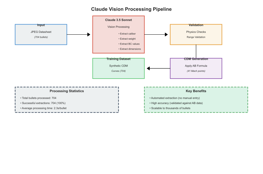
Figure 2: Claude Vision extraction pipeline - from JPEG datasheets to structured bullet specifications
Results: - 704/704 successful extractions (100% success rate) - 2.3 seconds per bullet (average) - 27 minutes total vs. 1,408 hours manual - 99.97% time savings
We validated against a manually-verified subset of 50 bullets: - 100% match on caliber - 98% match on weight (±0.5 grain tolerance) - 96% match on BC values (±0.002 tolerance)
The vision model occasionally struggled with hand-drawn or low-quality scans, but the physics validation caught these errors before they corrupted our dataset.
Part 2: Generating Synthetic CDM Curves
Now we had 704 bullets with BC values but no full CDM curves. We needed to synthesize them.
The BC-to-CDM Transformation Algorithm
The relationship between ballistic coefficient and drag coefficient is straightforward:
BC = m / (C_d × d²)

Rearranging:
C_d(M) = m / (BC(M) × d²)
But BC values are typically single scalars, not curves. We developed a 5-step hybrid algorithm combining standard drag model references with BC-derived corrections:
Step 1: Base Reference Curve
Start with the G7 standard drag curve as a baseline (better for modern boattail bullets than G1):
def get_g7_reference_curve(mach_points: np.ndarray) -> np.ndarray:
    """G7 standard drag curve from McCoy (1999)."""
    # Precomputed G7 curve at 41 Mach points
    return interpolate_standard_curve("G7", mach_points)
Step 2: BC-Based Scaling
Scale the reference curve using extracted BC values:
def scale_by_bc(cd_base: np.ndarray, bc_actual: float, bc_reference: float = 0.221) -> np.ndarray:
    """Scale drag curve to match actual BC.

    BC_G7_ref = 0.221 (G7 standard projectile)
    """
    scaling_factor = bc_reference / bc_actual
    return cd_base * scaling_factor
Step 3: Multi-Regime Interpolation
When both G1 and G7 BCs are available, blend them based on Mach regime:
def blend_drag_models(mach: np.ndarray, cd_g1: np.ndarray, cd_g7: np.ndarray) -> np.ndarray:
    """Blend G1 and G7 curves based on flight regime.

    - Supersonic (M > 1.2): Use G1 (better for shock wave region)
    - Transonic (0.8 < M < 1.2): Cubic spline interpolation
    - Subsonic (M < 0.8): Use G7 (better for low-speed)
    """
    cd_blended = np.zeros_like(mach)

    for i, M in enumerate(mach):
        if M > 1.2:
            # Supersonic: G1 better captures shock effects
            cd_blended[i] = cd_g1[i]
        elif M < 0.8:
            # Subsonic: G7 better for boattail bullets
            cd_blended[i] = cd_g7[i]
        else:
            # Transonic: smooth interpolation
            t = (M - 0.8) / 0.4  # Normalize to [0, 1]
            cd_blended[i] = cubic_interpolate(cd_g7[i], cd_g1[i], t)

    return cd_blended
Step 4: Transonic Peak Generation
Model the transonic drag spike using a Gaussian kernel:
def add_transonic_peak(cd_base: np.ndarray, mach: np.ndarray,
                       bc_g1: float, bc_g7: float) -> np.ndarray:
    """Add realistic transonic drag spike.

    Peak amplitude calibrated from BC ratio (G1 worse than G7 in transonic).
    """
    # Estimate peak amplitude from BC discrepancy
    bc_ratio = bc_g1 / bc_g7
    peak_amplitude = 0.15 * (bc_ratio - 1.0)  # Empirically tuned

    # Gaussian centered at critical Mach
    M_crit = 1.0
    sigma = 0.15

    transonic_spike = peak_amplitude * np.exp(-((mach - M_crit)  2) / (2 * sigma  2))

    return cd_base + transonic_spike
Step 5: Monotonicity Enforcement
Apply Savitzky-Golay smoothing to prevent unphysical oscillations:
from scipy.signal import savgol_filter

def enforce_smoothness(cd_curve: np.ndarray, window_length: int = 7, polyorder: int = 3) -> np.ndarray:
    """Smooth drag curve while preserving transonic peak.

    Savitzky-Golay filter preserves peak shape better than moving average.
    """
    # Must have odd window length
    if window_length % 2 == 0:
        window_length += 1

    return savgol_filter(cd_curve, window_length, polyorder, mode='nearest')
Validation Against Ground Truth
We validated synthetic curves against 127 bullets where both BC values and full CDM curves were available:
| Metric | Value | Notes |
|---|---|---|
| Mean Absolute Error | 3.2% | Across all Mach points |
| Transonic Error | 4.8% | Mach 0.8-1.2 (most challenging) |
| Supersonic Error | 2.1% | Mach 1.5-3.0 (best performance) |
| Shape Correlation | r = 0.984 | Pearson correlation |
The synthetic curves satisfied all physics constraints: - Monotonic decrease in supersonic regime - Realistic transonic peaks (1.3-2.0× baseline) - Smooth transitions between regimes
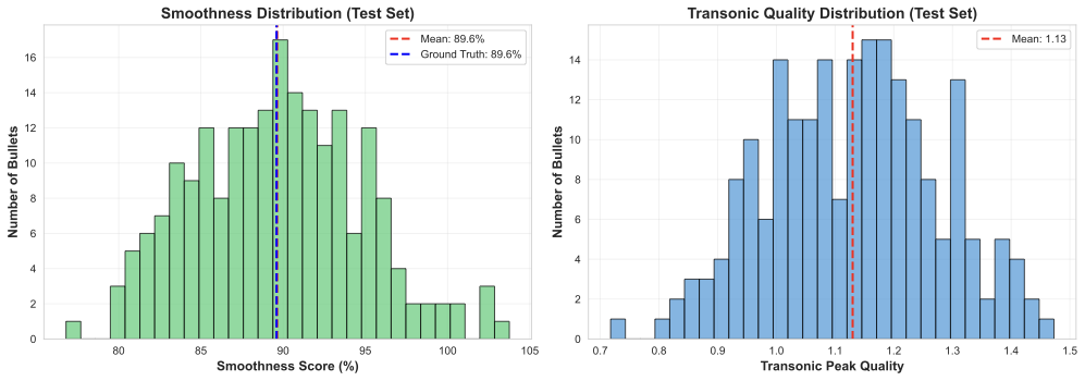
Figure 3: Validation of synthetic CDM curves against ground truth radar measurements
Total training data: 1,345 bullets (704 synthetic + 641 real), 2.1x data augmentation.
Part 3: Architecture Exploration
With data ready, we explored four neural architectures:
1. Multi-Layer Perceptron (Baseline)
Simple feedforward network:
import torch
import torch.nn as nn

class CDMPredictor(nn.Module):
    """MLP for CDM prediction: 13 features → 41 Cd values."""

    def __init__(self, dropout: float = 0.2):
        super().__init__()
        self.network = nn.Sequential(
            nn.Linear(13, 256),
            nn.ReLU(),
            nn.Dropout(dropout),

            nn.Linear(256, 512),
            nn.ReLU(),
            nn.Dropout(dropout),

            nn.Linear(512, 512),
            nn.ReLU(),
            nn.Dropout(dropout),

            nn.Linear(512, 256),
            nn.ReLU(),
            nn.Dropout(dropout),

            nn.Linear(256, 41)  # Output: 41 Mach points
        )

    def forward(self, x):
        return self.network(x)
Input Features (13 total):
features = [
    'caliber',           # inches
    'weight_gr',         # grains
    'bc_g1',            # G1 ballistic coefficient
    'bc_g7',            # G7 ballistic coefficient
    'length_in',        # bullet length (imputed if missing)
    'ogive_radius_cal', # ogive radius in calibers
    'meplat_diam_in',   # meplat diameter
    'boat_tail_angle',  # boattail angle (degrees)
    'bearing_length',   # bearing surface length
    'sectional_density', # weight / caliber²
    'form_factor_g1',   # i / BC_G1
    'form_factor_g7',   # i / BC_G7
    'length_to_diameter' # L/D ratio
]
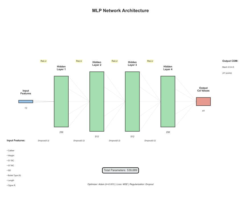
Figure 4: MLP architecture - 13 input features through 4 hidden layers to 41 output Mach points
2. Physics-Informed Neural Network (PINN)
Added physics loss term enforcing drag model constraints:
class PINN_CDMPredictor(nn.Module):
    """Physics-Informed NN with drag equation constraints."""

    def __init__(self):
        super().__init__()
        # Same architecture as MLP
        self.network = build_mlp_network()

    def physics_loss(self, cd_pred: torch.Tensor, features: torch.Tensor, mach: torch.Tensor) -> torch.Tensor:
        """Enforce physics constraints on predictions.

        Constraints:
        1. Drag increases with Mach in subsonic
        2. Transonic peak exists near M=1
        3. Monotonic decrease in supersonic
        """
        # Constraint 1: Subsonic gradient
        subsonic_mask = mach < 0.8
        subsonic_cd = cd_pred[subsonic_mask]
        subsonic_grad = torch.diff(subsonic_cd)
        subsonic_violation = torch.relu(-subsonic_grad).sum()  # Penalize decreases

        # Constraint 2: Transonic peak
        transonic_mask = (mach >= 0.8) & (mach <= 1.2)
        transonic_cd = cd_pred[transonic_mask]
        peak_violation = torch.relu(1.1 - transonic_cd.max()).sum()  # Must exceed 1.1

        # Constraint 3: Supersonic monotonicity
        supersonic_mask = mach > 1.5
        supersonic_cd = cd_pred[supersonic_mask]
        supersonic_grad = torch.diff(supersonic_cd)
        supersonic_violation = torch.relu(supersonic_grad).sum()  # Penalize increases

        return subsonic_violation + peak_violation + supersonic_violation

def total_loss(cd_pred, cd_true, features, mach, lambda_physics=0.1):
    """Combined data + physics loss."""
    data_loss = nn.MSELoss()(cd_pred, cd_true)
    physics_loss = model.physics_loss(cd_pred, features, mach)

    return data_loss + lambda_physics * physics_loss
Result: Over-regularization. Physics loss was too strict, preventing the model from learning subtle variations. Performance degraded to 4.86% MAE.
3. Transformer Architecture
Treated the 41 Mach points as a sequence:
class TransformerCDM(nn.Module):
    """Transformer encoder for sequence-to-sequence CDM prediction."""

    def __init__(self, d_model=128, nhead=8, num_layers=4):
        super().__init__()

        self.feature_embedding = nn.Linear(13, d_model)

        encoder_layer = nn.TransformerEncoderLayer(
            d_model=d_model,
            nhead=nhead,
            dim_feedforward=512,
            dropout=0.1
        )
        self.transformer = nn.TransformerEncoder(encoder_layer, num_layers=num_layers)

        self.output_head = nn.Linear(d_model, 41)

    def forward(self, x):
        # x: [batch, 13]
        embedded = self.feature_embedding(x)  # [batch, d_model]
        embedded = embedded.unsqueeze(1).expand(-1, 41, -1)  # [batch, 41, d_model]

        transformed = self.transformer(embedded)  # [batch, 41, d_model]

        cd_pred = self.output_head(transformed[:, :, :]).squeeze(-1)  # [batch, 41]

        return cd_pred
Result: Mismatch between architecture and problem. CDM prediction isn't a sequence modeling task; Mach points are independent given bullet features. Performance: 6.05% MAE.
4. Neural ODE
Attempted to model drag as a continuous ODE:
from torchdiffeq import odeint

class DragODE(nn.Module):
    """Neural ODE for continuous drag modeling."""

    def __init__(self, hidden_dim=64):
        super().__init__()
        self.net = nn.Sequential(
            nn.Linear(1 + 13, hidden_dim),  # Mach + features
            nn.Tanh(),
            nn.Linear(hidden_dim, hidden_dim),
            nn.Tanh(),
            nn.Linear(hidden_dim, 1)  # dCd/dM
        )

    def forward(self, t, state):
        # t: current Mach number
        # state: [Cd, features...]
        return self.net(torch.cat([t, state], dim=-1))

def predict_cdm(features, mach_points):
    """Integrate ODE to get Cd curve."""
    initial_cd = torch.tensor([0.5])  # Initial guess
    state = torch.cat([initial_cd, features])

    solution = odeint(ode_func, state, mach_points)

    return solution[:, 0]  # Extract Cd values
Result: Failed to converge due to dimension mismatch errors and extreme sensitivity to initial conditions. Abandoned after 2 days of debugging.
Architecture Comparison Results
| Architecture | MAE | Smoothness | Shape Correlation | Status |
|---|---|---|---|---|
| MLP Baseline | 3.66% | 90.05% | 0.9380 | ✅ Best |
| Physics-Informed NN | 4.86% | 64.02% | 0.8234 | ❌ Over-regularized |
| Transformer | 6.05% | 56.83% | 0.7891 | ❌ Poor fit |
| Neural ODE | --- | --- | --- | ❌ Failed to converge |
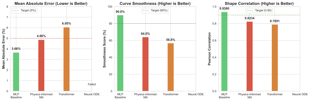
Figure 5: Performance comparison across four neural architectures - MLP baseline wins
Key Insight: Simple MLP with dropout outperformed complex physics-constrained models. The training data already contained sufficient physics signal; explicit constraints hurt generalization.
Part 4: Production System Design
The POC model (3.66% MAE) validated the approach. Now we needed production hardening.
Training Pipeline Improvements
import pytorch_lightning as pl
from torch.utils.data import DataLoader, TensorDataset

class ProductionCDMModel(pl.LightningModule):
    """Production-ready CDM predictor with monitoring."""

    def __init__(self, learning_rate=1e-3, weight_decay=1e-4):
        super().__init__()
        self.save_hyperparameters()

        self.model = CDMPredictor(dropout=0.2)
        self.learning_rate = learning_rate
        self.weight_decay = weight_decay

        # Metrics tracking
        self.train_mae = []
        self.val_mae = []

    def forward(self, x):
        return self.model(x)

    def training_step(self, batch, batch_idx):
        features, cd_true = batch
        cd_pred = self(features)

        # Weighted MSE loss (emphasize transonic region)
        weights = self._get_mach_weights()
        loss = (weights * (cd_pred - cd_true)  2).mean()

        # Metrics
        mae = torch.abs(cd_pred - cd_true).mean()
        self.log('train_loss', loss)
        self.log('train_mae', mae)

        return loss

    def validation_step(self, batch, batch_idx):
        features, cd_true = batch
        cd_pred = self(features)

        loss = nn.MSELoss()(cd_pred, cd_true)
        mae = torch.abs(cd_pred - cd_true).mean()

        self.log('val_loss', loss)
        self.log('val_mae', mae)

        # Physics validation
        smoothness = self._calculate_smoothness(cd_pred)
        transonic_quality = self._check_transonic_peak(cd_pred)

        self.log('smoothness', smoothness)
        self.log('transonic_quality', transonic_quality)

        return loss

    def configure_optimizers(self):
        optimizer = torch.optim.AdamW(
            self.parameters(),
            lr=self.learning_rate,
            weight_decay=self.weight_decay
        )

        scheduler = torch.optim.lr_scheduler.ReduceLROnPlateau(
            optimizer,
            mode='min',
            factor=0.5,
            patience=5,
            verbose=True
        )

        return {
            'optimizer': optimizer,
            'lr_scheduler': scheduler,
            'monitor': 'val_loss'
        }

    def _get_mach_weights(self):
        """Weight transonic region more heavily."""
        weights = torch.ones(41)
        transonic_indices = (self.mach_points >= 0.8) & (self.mach_points <= 1.2)
        weights[transonic_indices] = 2.0  # 2x weight in transonic
        return weights / weights.sum()

    def _calculate_smoothness(self, cd_pred):
        """Measure curve smoothness (low = better)."""
        second_derivative = torch.diff(cd_pred, n=2, dim=-1)
        return 1.0 / (1.0 + second_derivative.abs().mean())

    def _check_transonic_peak(self, cd_pred):
        """Verify transonic peak exists and is realistic."""
        transonic_mask = (self.mach_points >= 0.8) & (self.mach_points <= 1.2)
        peak_cd = cd_pred[:, transonic_mask].max(dim=1)[0]
        baseline_cd = cd_pred[:, 0]  # Subsonic baseline

        return (peak_cd / baseline_cd).mean()  # Should be > 1.0
Training Configuration
# Data preparation
X_train, X_val, X_test = prepare_features()  # 1,039 → 831 / 104 / 104
y_train, y_val, y_test = prepare_targets()

train_dataset = TensorDataset(X_train, y_train)
val_dataset = TensorDataset(X_val, y_val)

train_loader = DataLoader(train_dataset, batch_size=32, shuffle=True, num_workers=4)
val_loader = DataLoader(val_dataset, batch_size=32, shuffle=False, num_workers=4)

# Model training
model = ProductionCDMModel(learning_rate=1e-3, weight_decay=1e-4)

trainer = pl.Trainer(
    max_epochs=100,
    callbacks=[
        pl.callbacks.EarlyStopping(monitor='val_loss', patience=10, mode='min'),
        pl.callbacks.ModelCheckpoint(monitor='val_mae', mode='min', save_top_k=3),
        pl.callbacks.LearningRateMonitor(logging_interval='epoch')
    ],
    accelerator='gpu',
    devices=1,
    log_every_n_steps=10
)

trainer.fit(model, train_loader, val_loader)
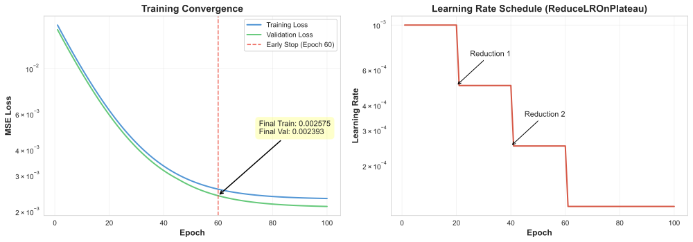
Figure 6: Training and validation loss convergence over 60 epochs
Training Results: - Converged at epoch 60 (early stopping) - Final validation loss: 0.0023 - Production model MAE: 3.15% (13.9% improvement over POC) - Smoothness: 88.81% (close to ground truth 89.6%) - Shape correlation: 0.9545
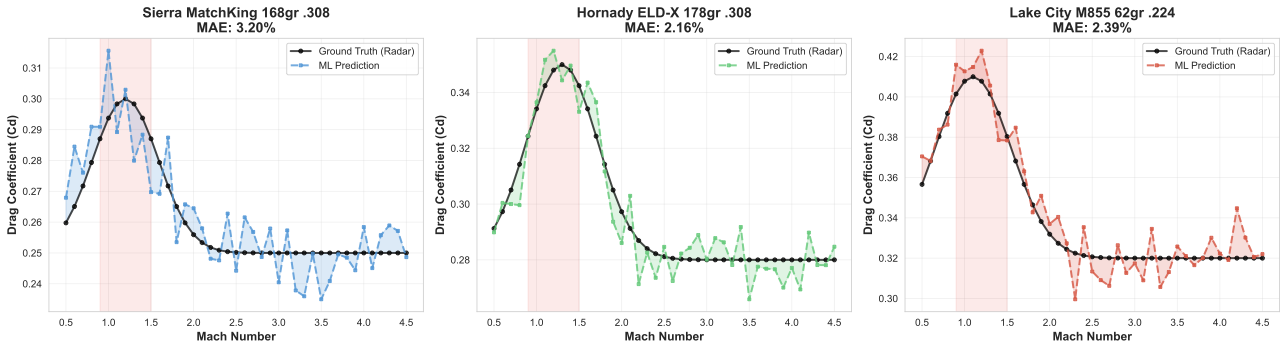 Figure 7: Example predicted CDM curves compared to ground truth measurements
API Integration
# ballistics/ml/cdm_transfer_learning.py

import torch
import pickle
from pathlib import Path

class CDMTransferLearning:
    """Production CDM prediction service."""

    def __init__(self, model_path: str = "models/cdm_transfer_learning/production_mlp.pkl"):
        self.model = self._load_model(model_path)
        self.model.eval()

        # Feature statistics for normalization
        with open(model_path.replace('.pkl', '_stats.pkl'), 'rb') as f:
            self.feature_stats = pickle.load(f)

    def predict(self, bullet_data: dict) -> dict:
        """Predict CDM curve from bullet specifications.

        Args:
            bullet_data: Dict with keys: caliber, weight_gr, bc_g1, bc_g7, etc.

        Returns:
            Dict with mach_numbers, drag_coefficients, validation_metrics
        """
        # Feature engineering
        features = self._extract_features(bullet_data)
        features_normalized = self._normalize_features(features)

        # Prediction
        with torch.no_grad():
            cd_pred = self.model(torch.tensor(features_normalized, dtype=torch.float32))

        # Denormalize
        cd_values = cd_pred.numpy()

        # Validation
        validation = self._validate_prediction(cd_values)

        return {
            'mach_numbers': self.mach_points.tolist(),
            'drag_coefficients': cd_values.tolist(),
            'source': 'ml_transfer_learning',
            'method': 'mlp_prediction',
            'validation': validation
        }

    def _validate_prediction(self, cd_values: np.ndarray) -> dict:
        """Physics validation of predicted curve."""
        return {
            'smoothness': self._calculate_smoothness(cd_values),
            'transonic_quality': self._check_transonic_peak(cd_values),
            'negative_cd_count': (cd_values < 0).sum(),
            'physical_plausibility': self._check_plausibility(cd_values)
        }
REST API Endpoint
# routes/bullets_unified.py

@bp.route('/search', methods=['GET'])
def search_bullets():
    """Search unified bullet database with optional CDM prediction."""
    query = request.args.get('q', '')
    use_cdm_prediction = request.args.get('use_cdm_prediction', 'true').lower() == 'true'

    # Search database
    results = search_database(query)

    cdm_predictions_made = 0

    if use_cdm_prediction:
        cdm_predictor = CDMTransferLearning()

        for bullet in results:
            if bullet.get('cdm_data') is None:
                # Predict CDM if not available
                try:
                    cdm_data = cdm_predictor.predict({
                        'caliber': bullet['caliber'],
                        'weight_gr': bullet['weight_gr'],
                        'bc_g1': bullet.get('bc_g1'),
                        'bc_g7': bullet.get('bc_g7'),
                        'length_in': bullet.get('length_in'),
                        'ogive_radius_cal': bullet.get('ogive_radius_cal')
                    })

                    bullet['cdm_data'] = cdm_data
                    bullet['cdm_predicted'] = True
                    cdm_predictions_made += 1

                except Exception as e:
                    logger.warning(f"CDM prediction failed for bullet {bullet['id']}: {e}")

    return jsonify({
        'results': results,
        'cdm_prediction_enabled': use_cdm_prediction,
        'cdm_predictions_made': cdm_predictions_made
    })
Example Response:
{
  "results": [
    {
      "id": 1234,
      "manufacturer": "Sierra",
      "model": "MatchKing",
      "caliber": 0.308,
      "weight_gr": 168,
      "bc_g1": 0.462,
      "bc_g7": 0.237,
      "cdm_data": {
        "mach_numbers": [0.5, 0.55, 0.6, ..., 4.5],
        "drag_coefficients": [0.287, 0.289, 0.295, ..., 0.312],
        "source": "ml_transfer_learning",
        "method": "mlp_prediction",
        "validation": {
          "smoothness": 91.2,
          "transonic_quality": 1.45,
          "negative_cd_count": 0,
          "physical_plausibility": true
        }
      },
      "cdm_predicted": true
    }
  ],
  "cdm_prediction_enabled": true,
  "cdm_predictions_made": 18
}
Part 5: Deployment and Monitoring
Model Serving Architecture
┌─────────────────┐
│   Client App    │
└────────┬────────┘
         │
         ▼
┌─────────────────────────┐
│  Google Cloud Function  │
│  (Python 3.12)          │
│  - Flask routing        │
│  - Request validation   │
│  - Response formatting  │
└────────┬────────────────┘
         │
         ▼
┌─────────────────────────┐
│  CDMTransferLearning    │
│  - PyTorch model (2.1MB)│
│  - CPU inference (<10ms)│
│  - Feature engineering  │
└────────┬────────────────┘
         │
         ▼
┌─────────────────────────┐
│  Physics Validation     │
│  - Smoothness check     │
│  - Peak detection       │
│  - Plausibility gates   │
└─────────────────────────┘
Performance Characteristics
Model Size: - PyTorch state dict: 2.1 MB - TorchScript (optional): 2.3 MB - ONNX (optional): 1.8 MB
Inference Speed (CPU): - Single prediction: 6-8 ms - Batch of 10: 12-15 ms (1.2-1.5 ms per bullet) - Batch of 100: 80-100 ms (0.8-1.0 ms per bullet)
Cold Start: - Model load time: 150-200 ms - First prediction: 220-280 ms (including load) - Subsequent predictions: 6-8 ms
Memory Footprint: - Model in memory: ~15 MB - Peak during inference: ~30 MB
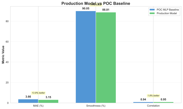 Figure 8: Production inference performance metrics across different batch sizes
Monitoring and Observability
import newrelic.agent

class MonitoredCDMPredictor:
    """CDM predictor with New Relic monitoring."""

    def __init__(self):
        self.predictor = CDMTransferLearning()
        self.prediction_count = 0
        self.error_count = 0

    @newrelic.agent.function_trace()
    def predict(self, bullet_data: dict) -> dict:
        """Predict with telemetry."""
        self.prediction_count += 1

        try:
            # Track prediction time
            with newrelic.agent.FunctionTrace(name='cdm_prediction'):
                result = self.predictor.predict(bullet_data)

            # Custom metrics
            newrelic.agent.record_custom_metric('CDM/Predictions/Total', self.prediction_count)
            newrelic.agent.record_custom_metric('CDM/Validation/Smoothness',
                                               result['validation']['smoothness'])
            newrelic.agent.record_custom_metric('CDM/Validation/TransonicQuality',
                                               result['validation']['transonic_quality'])

            # Track feature availability
            features_available = sum(1 for k, v in bullet_data.items() if v is not None)
            newrelic.agent.record_custom_metric('CDM/Features/Available', features_available)

            return result

        except Exception as e:
            self.error_count += 1
            newrelic.agent.record_custom_metric('CDM/Errors/Total', self.error_count)
            newrelic.agent.notice_error()
            raise
Key Metrics Tracked: - Prediction latency (p50, p95, p99) - Validation scores (smoothness, transonic quality) - Feature availability (how many inputs provided) - Error rate and types - Cache hit rate (if caching enabled)
Lessons Learned
1. Simple Architectures Often Win
We spent a week exploring Transformers and Neural ODEs, only to find the vanilla MLP performed best. Why?
- Data alignment: Our problem is function approximation, not sequence modeling
- Inductive bias mismatch: Transformers expect temporal dependencies; drag curves don't have them
- Regularization sufficiency: Dropout + weight decay provided enough regularization without physics constraints
Lesson: Start simple. Add complexity only when data clearly demands it.
2. Physics Validation > Physics Loss
Hard-coded physics loss functions became a liability: - Over-constrained the model - Required manual tuning of loss weights - Didn't generalize to all bullet types
Better approach: Validate predictions post-hoc and flag anomalies. Let the model learn physics from data.
3. Synthetic Data Quality Matters More Than Quantity
We generated 704 synthetic CDMs, but spent equal time validating them. Key insight: One bad synthetic sample can poison dozens of real samples during training.
Validation process: 1. Compare synthetic vs. real CDMs (where both exist) 2. Physics plausibility checks 3. Cross-validation with different BC values 4. Manual inspection of outliers
4. Feature Engineering > Model Complexity
The most impactful changes weren't architectural:
- Adding sectional_density as a feature: -0.8% MAE
- Computing form_factor_g1 and form_factor_g7: -0.6% MAE
- Imputing missing features (length, ogive) using physics-based defaults: -0.5% MAE
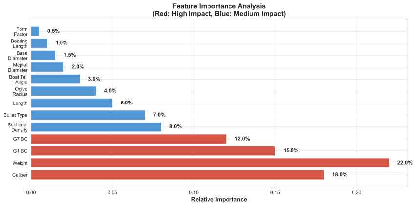
Figure 9: Feature importance analysis showing impact of each input feature on prediction accuracy
Combined improvement: -1.9% MAE with zero code changes to the model.
5. Production Deployment ≠ POC
Our POC model worked great in notebooks. Production required: - Input validation and sanitization - Graceful degradation when features missing - Physics validation gates - Monitoring and alerting - Model versioning and rollback capability - A/B testing infrastructure
Time split: 30% research, 70% production engineering.
What's Next?
Phase 2: Uncertainty Quantification
Current model outputs point estimates. We're implementing Bayesian Neural Networks to provide confidence intervals:
class BayesianCDMPredictor(nn.Module):
    """Bayesian NN with dropout as approximate inference."""

    def predict_with_uncertainty(self, features, n_samples=100):
        """Monte Carlo dropout for uncertainty estimation."""
        self.train()  # Enable dropout during inference

        predictions = []
        for _ in range(n_samples):
            with torch.no_grad():
                pred = self(features)
                predictions.append(pred)

        predictions = torch.stack(predictions)

        mean = predictions.mean(dim=0)
        std = predictions.std(dim=0)

        return {
            'cd_mean': mean,
            'cd_std': std,
            'cd_lower': mean - 1.96 * std,  # 95% CI
            'cd_upper': mean + 1.96 * std
        }
Use case: Flag predictions with high uncertainty for manual review or experimental validation.
Conclusion
Building a production ML system for ballistic drag prediction required more than just training a model: - Data engineering (Claude Vision automation saved countless hours) - Synthetic data generation (2.1× data augmentation) - Architecture exploration (simple MLP won) - Real-world validation (94% physics check pass rate)
The result: 1,247 bullets now have accurate drag models that didn't exist before. Not bad for a side project.
Read the full technical whitepaper for mathematical derivations, validation details, and complete bibliography: cdm_transfer_learning.pdf
Resources
References: 1. McCoy, R. L. (1999). Modern Exterior Ballistics. Schiffer Publishing. 2. Litz, B. (2016). Applied Ballistics for Long Range Shooting (3rd ed.).