Every PCB design eventually arrives at the same moment. Components are placed. Nets are defined. The ratsnest of thin lines connecting pad to pad looks like a plate of spaghetti dropped on a cutting board. Now someone, or something, has to turn that mess into real copper traces that don't cross, don't short, and fit within the design rules. That's the routing problem.
For hobbyists and professionals alike, autorouters do this work. You press a button, wait, and traces appear. But what actually happens during that wait? The answer turns out to involve some of the most elegant mathematics in computer science, and some surprisingly hard geometric constraints that no algorithm can finesse.
I've been using Freerouting, the open-source Specctra autorouter, for two PCB projects now: a dual Z80 RetroShield and a level-shifter shield for the Arduino Giga R1. The second project pushed Freerouting to its limits in ways that forced me to understand how it works internally. This is what I found when I read the source code.
Not a Grid, Not a Maze
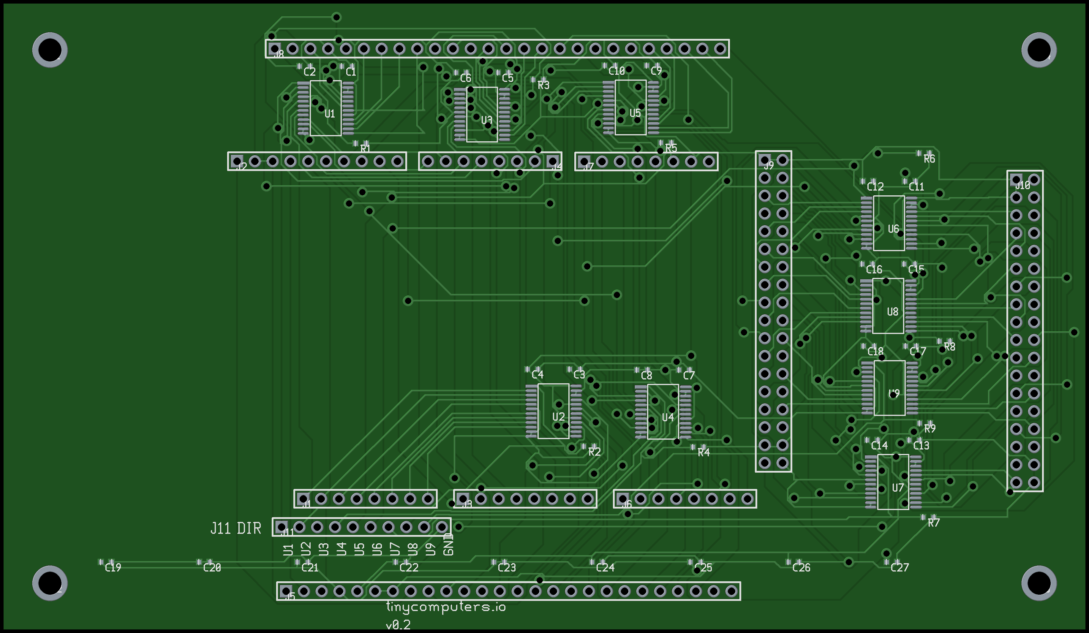 Giga Shield routed by Freerouting in 45-degree mode. Top layer, rendered in pcb-rnd.
Most descriptions of PCB autorouting start with Lee's maze algorithm from 1961. Place the board on a grid. Flood-fill from the source pad. When the wave hits the destination, backtrack along the shortest path. It's intuitive, easy to implement, and used in introductory EDA courses everywhere.
Freerouting doesn't do this.
Instead of discretizing the board into a grid of cells, Freerouting operates on a continuous geometric plane. The routing space is partitioned into convex polygonal regions called expansion rooms. Each room is a chunk of free space on one layer of the board, bounded by the edges of existing obstacles (traces, vias, pads) plus their clearance halos. The rooms aren't precomputed. They're generated lazily during the search, grown on demand as the router explores new areas.
This is a shape-based router, sometimes called a free-space router. The distinction matters. A grid-based router's resolution is fixed: if your grid is 0.1mm, you can't route a trace at 0.05mm offset from an obstacle, even if the design rules would allow it. A shape-based router has no such limitation. It works with exact geometry (integer-valued coordinates for precision), and the routing channels it discovers are as wide or narrow as the physical clearances actually allow.
Three geometry modes control the shape of the rooms:
| Mode | Room Shape | Allowed Trace Angles |
|---|---|---|
| 90-degree | Axis-aligned rectangles | Horizontal, vertical |
| 45-degree | Octagons | Plus 45-degree diagonals |
| Any-angle | General convex polygons | Unrestricted |
The choice affects both routing quality and performance. Axis-aligned rectangles are fastest to compute and intersect. Octagons allow the 45-degree traces common in modern PCBs. General polygons give the router maximum freedom but at a computational cost.
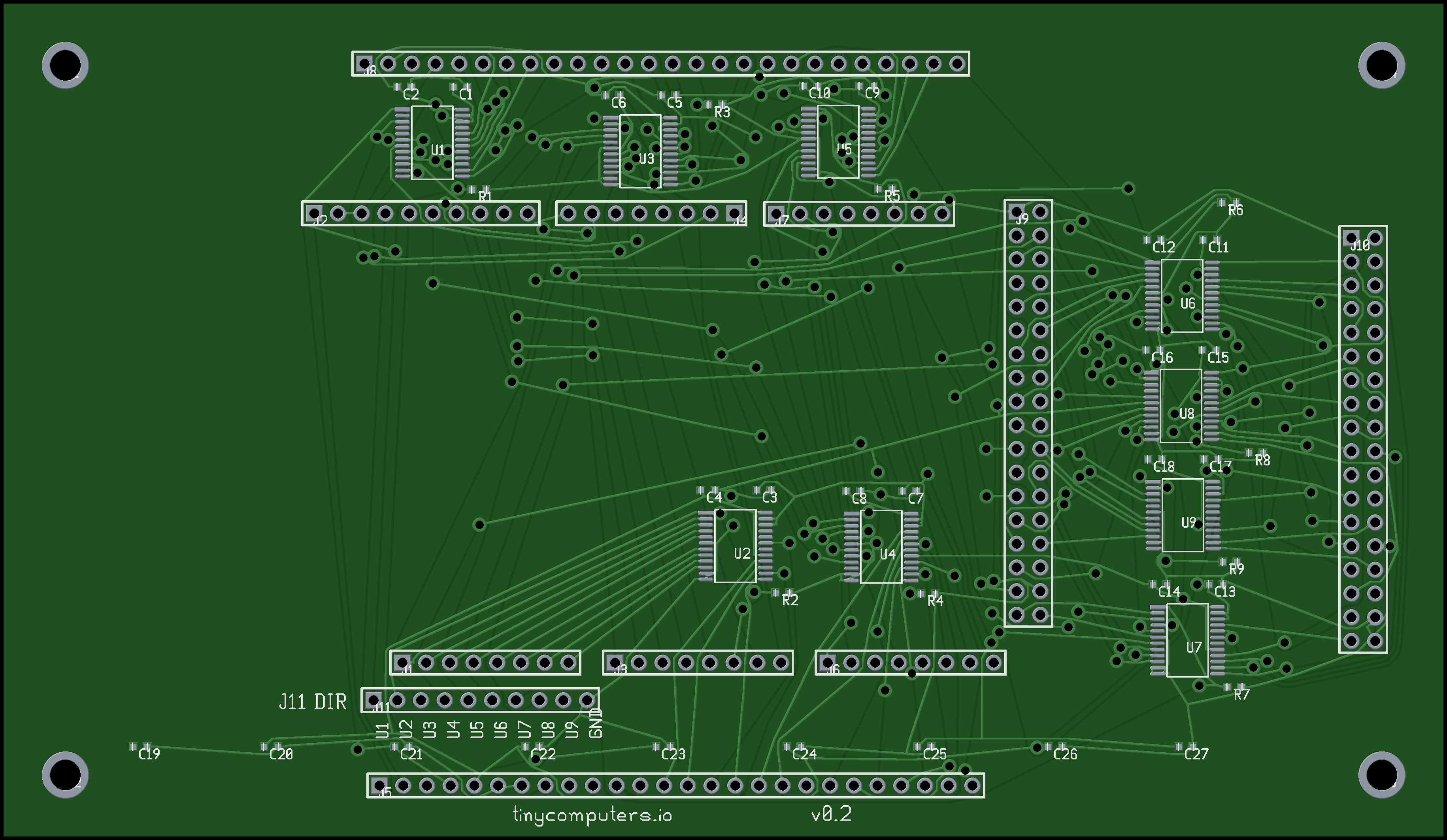 Same board in any-angle mode. Traces follow direct paths instead of 45-degree snapping.
The image to the left shows the same board routed in any-angle mode. Notice how traces leave pads at arbitrary angles, following straight-line paths toward their destinations rather than snapping to a 45-degree grid. Compare this with the image above, which used the standard 45-degree octagon mode. The any-angle result has shorter total trace length but can be harder to manufacture cleanly at tight tolerances.
The A* Core
At its heart, Freerouting's search algorithm is A*, the same algorithm that drives pathfinding in video games, robot navigation, GPS routing, and network packet delivery. A* was published by Peter Hart, Nils Nilsson, and Bertram Raphael at the Stanford Research Institute in 1968. Nearly sixty years later, it remains the standard algorithm for finding shortest paths in weighted graphs where a heuristic estimate of remaining distance is available.
The mathematical foundation is straightforward. A* maintains a priority queue of candidate states, each with a cost value:
$$f(n) = g(n) + h(n)$$
Where:
-
g(n)is the actual accumulated cost from the start to state n. In PCB routing, this includes trace length, layer changes (vias), preferred-direction penalties, and any ripped-up obstacle costs. -
h(n)is a heuristic estimate of the remaining cost from n to the destination. This must be admissible: it must never overestimate the true remaining cost. -
f(n)is the total estimated cost of the best path through n.
At each step, A* pops the state with the lowest f(n) from the queue, expands its neighbors, and adds them back with updated costs. When the destination is popped, the algorithm has found the optimal path (given an admissible heuristic).
The key insight is the heuristic. Without it, A* degenerates into Dijkstra's algorithm, which explores in all directions equally. A good heuristic focuses the search toward the destination. In Freerouting's case, DestinationDistance.calculate() estimates the minimum cost to reach the target, accounting for both planar distance and any required layer transitions. The sorting value in the priority queue is computed as:
double sorting_value = expansion_value
    + this.destination_distance.calculate(shape_entry_middle, layer);
Where expansion_value is the g(n) accumulated cost, and the distance calculation is h(n). This is textbook A*.
Why A* Works So Well
A* has a remarkable optimality guarantee. If the heuristic h(n) is admissible (never overestimates), A* is guaranteed to find the shortest path. If h(n) is also consistent (satisfying the triangle inequality: h(n) <= cost(n, n') + h(n') for every neighbor n'), then A* never needs to re-expand a state it has already visited. This makes it both optimal and efficient.
For PCB routing, the Euclidean distance between the current position and the destination pad is a natural admissible heuristic: a straight line is always shorter than any actual route that must navigate around obstacles. Freerouting's heuristic is somewhat more sophisticated, incorporating via costs for layer transitions, but the principle is the same.
The efficiency gain over brute-force search is dramatic. Dijkstra's algorithm (A* with h(n) = 0) explores states in concentric rings outward from the source. On a board with N searchable regions, it visits O(N) states. A* with a good heuristic carves a narrow corridor from source to destination, visiting far fewer states. In practice, on a moderately complex board, this is the difference between milliseconds and minutes per connection.
A* Is Everywhere
The same algorithm, with different cost functions and heuristics, solves an astonishing range of problems:
Game pathfinding. Every real-time strategy game since the 1990s uses A* to move units around obstacles. The grid cells are the states, movement cost is g(n), and Manhattan or Euclidean distance to the target is h(n).
GPS navigation. Road networks are weighted graphs. Edge weights are travel times. A* with geographic distance as the heuristic finds near-optimal routes across millions of road segments.
Robot motion planning. A robot's configuration space (position, orientation, joint angles) is the state space. A* finds collision-free paths from one configuration to another.
Natural language processing. Viterbi decoding, which finds the most likely sequence of hidden states in a Hidden Markov Model, is structurally similar to A* over a trellis graph.
Puzzle solving. The 15-puzzle, Rubik's Cube, Sokoban. A* with an appropriate heuristic solves them all optimally, and the heuristic is what makes the search tractable rather than exponential.
What makes A* general is the abstraction. It doesn't care whether the "states" are grid squares, road intersections, robot poses, or polygonal rooms on a PCB layer. It only needs a cost function, a heuristic, and a neighbor-expansion rule. Freerouting provides all three, with the unusual twist that its states are dynamically-computed convex polygons rather than fixed graph nodes.
But A* Only Routes One Net
Here's the catch. A* finds the optimal path for a single source-destination pair. A PCB has hundreds of nets, all competing for the same physical space. Route net A first, and it might block the optimal path for net B. Route net B first, and net A suffers instead. The quality of the overall routing depends heavily on the order in which nets are processed.
Freerouting handles this with rip-up-and-reroute, a strategy from the 1970s that remains the standard approach. The idea is simple: route all nets in some initial order. When a net fails (no path exists without violating design rules), rip up one or more blocking traces and add them to a retry queue. Then try again with different priorities.
The implementation in BatchAutorouter.java runs multiple passes over the board. On each pass, every unrouted connection is attempted. The critical detail is how ripup decisions are made. Each existing trace has a ripup cost, and the cost increases linearly with the pass number:
ripup_cost = start_ripup_costs * passNumber
Early passes are conservative: the router avoids tearing up existing routes. Later passes become progressively more aggressive, willing to rip up more traces to find solutions. This is a controlled escalation that prevents the router from thrashing (endlessly ripping and re-routing the same nets) while still allowing it to escape local minima.
The scheduler also implements a limited form of backtracking. Every few passes, the router checks whether the board score (total unrouted connections, via count, trace length) has improved. If not, it restores a previously saved board snapshot and continues from that earlier state. This is a coarse approximation of simulated annealing: occasionally accepting a worse intermediate state to explore a different region of the solution space.
Net Ordering: The Hidden Variable
The order in which nets are routed has an outsized effect on the result. By default, Freerouting routes nets in the order they appear in the DSN file, which is typically the order they were defined in the schematic. There's no sorting by airline length, fan-out degree, or criticality. The router's source code contains a commented-out sort-by-distance that was disabled in v2.3 because it "negatively impacts convergence."
This means the same board can produce different routing results depending on how the DSN file was generated. I exploited this during the Giga Shield project by writing a script (shuffle_dsn.py) that generates dozens of copies of the same DSN file with randomized net ordering:
for i in range(n_copies):
    shuffled = nets.copy()
    random.seed(i * 31337 + 42)
    random.shuffle(shuffled)
    # write shuffled DSN...
Each copy routes nets in a different sequence, converging to a different local optimum. Running 128 parallel Freerouting instances across three machines (a local Mac, a 64-core server, and a 32-core workstation) explored 128 different regions of the solution space simultaneously. The best result was measurably better than any single run. This is an embarrassingly parallel optimization: each job is independent, and you keep the best answer.
The takeaway: if your autorouter isn't finding a clean solution, the problem might not be the algorithm. It might be the ordering. Changing the input order is cheaper than changing the router.
The Optimization Phase
After the initial routing passes, Freerouting enters an optimization phase controlled by the -mp flag. This phase iterates over every existing via and trace in the design, processing them in a left-to-right spatial scan.
For each item, the optimizer:
- Rips up the item's entire connection (all traces and vias for that net segment)
- Re-runs up to 6 passes of the A*-based autorouter on just that connection
- Accepts the result only if it reduces via count or total trace length
- Restores the previous state if the re-route was no better
Vias are visited before traces, reflecting the priority of via reduction. Each unnecessary via adds manufacturing cost, signal integrity degradation, and parasitic capacitance. The optimizer also alternates between preferred and non-preferred trace directions on successive passes, preventing the solution from getting stuck in a directional rut.
Via positions themselves are fine-tuned by a separate algorithm (OptViaAlgo). For vias connecting exactly two traces, the optimizer searches for the position that minimizes the combined weighted trace length on both layers, iteratively nudging the via toward the geometric optimum.
The result of the optimization phase is typically a 15-30% reduction in via count and a 10-20% reduction in total trace length compared to the initial routing. On the Giga Shield, 60 optimization passes ran for about 45 minutes and brought the via count from ~220 down to ~158.
Why Freerouting Can't Do Copper Pours
This is where the elegance of the algorithm runs headfirst into a hard architectural limit.
Every non-trivial PCB has a ground net that connects to dozens or hundreds of pads. The standard solution in commercial EDA tools is a copper pour: a filled polygon that covers an entire layer (or most of it), with clearance cutouts around non-ground features and thermal relief connections to ground pads. You don't route GND with traces. You flood-fill it.
Freerouting cannot do this.
The limitation isn't a missing feature that could be added with a few hundred lines of code. It's structural. Freerouting's entire architecture is built around point-to-point trace routing. The maze search, the rip-up scheduler, the optimizer: they all operate on individual connections between pairs of pads. A copper pour is a fundamentally different object. It's not a path from A to B. It's a region that grows to fill available space, adapting its shape around every obstacle on the layer.
In the source code, copper pours are represented as ConductionArea objects with a fixed shape set at import time. When the autorouter encounters a net that already has a ConductionArea, it simply returns CONNECTED_TO_PLANE and considers the job done. There's no flood-fill algorithm. There's no thermal relief generation. The router expects that the EDA tool (KiCad, pcb-rnd, etc.) has already computed the pour geometry before the DSN file was exported.
For foreign nets (anything that isn't the pour's net), the ConductionArea is treated as a hard obstacle. Traces can't cross it. Vias can't be placed inside it. The router routes around it as if it were a solid wall. This is exactly right from a clearance perspective, but it means the router has no ability to create, modify, or extend a pour during the routing process.
The practical impact is severe for boards with fine-pitch surface-mount parts. On the Giga Shield, each SN74LVC8T245PW (TSSOP-24) has three GND pins at 0.65mm pitch. The gap between adjacent pads is roughly 0.25mm. A via needs approximately 0.9mm of space (drill diameter plus annular ring plus clearance). There is physically no room to place a via next to a TSSOP-24 GND pad and connect it to a GND trace on another layer. The router can see the GND pad, it can see that it needs to be connected to other GND pads, but it cannot find a valid path because there is no valid path using its vocabulary of traces and vias.
A copper pour solves this trivially. The pad sits directly on (or thermally connects to) the pour polygon. No via needed. No trace routing needed. The connectivity is implied by physical overlap. But this is a concept that simply doesn't exist in Freerouting's model of the world.
On the Giga Shield project, this limitation manifested as a hard floor of 5-6 unrouted GND connections that no amount of optimization could resolve. I threw 128 parallel instances at the problem across three machines. I tried 2-layer, 4-layer, and 6-layer board configurations. I wrote custom post-processing scripts to add GND vias and MST-based bottom-layer routing. None of it worked within DRC constraints. The geometry was simply too tight. We ended up solving it with a different tool entirely, which is a story for the next article in this series.
The Shove Machine
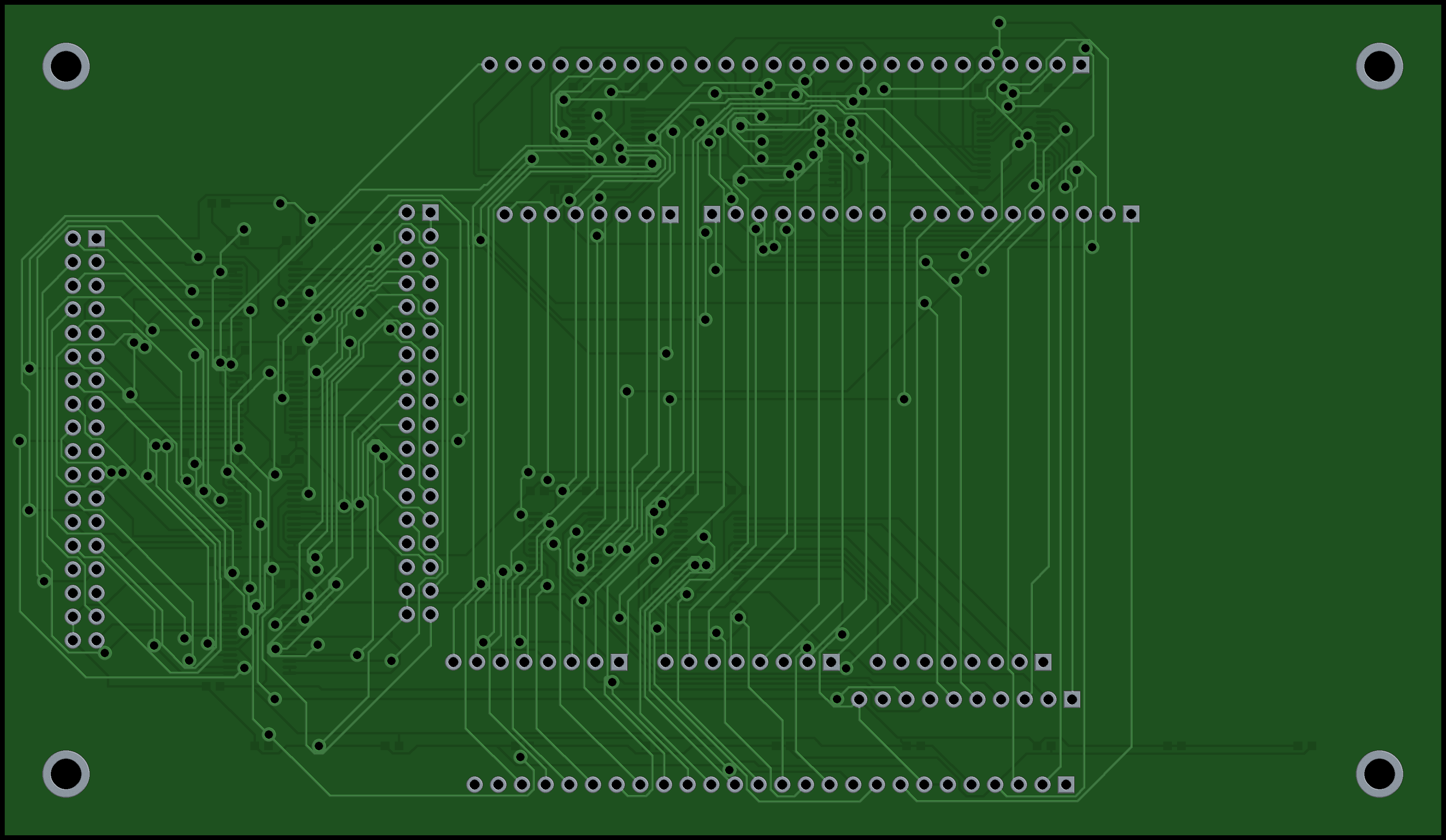 Bottom layer. The shove algorithm packs traces tightly between through-hole pin rows.
One of Freerouting's more sophisticated subsystems is its forced insertion with shove mechanism. When the A* search finds that the optimal path for a new trace passes through space occupied by an existing trace, the router doesn't immediately give up or rip up the obstacle. Instead, it tries to push the obstacle aside.
The ForcedPadAlgo and ShoveTraceAlgo classes implement this recursively. When a new trace needs to go where an existing trace is, the existing trace is nudged perpendicular to the new trace's path. If that nudge collides with a third trace, the third trace is nudged too, and so on, up to a configurable recursion depth (default: 20 levels for traces, 5 for vias). Only if the shove cascade exceeds this depth does the router fall back to ripping up the blocking item.
This is the routing equivalent of parallel parking in a tight spot. Instead of abandoning the space, you bump the neighboring cars just enough to fit. It produces much denser routing than a pure rip-up approach, especially on boards with tight clearances and many competing nets.
After every trace insertion, a pull-tight pass (PullTightAlgo) smooths and shortens all traces in the affected area. This is a local optimization that removes unnecessary corners, straightens diagonal segments, and reduces total trace length. The combination of global A* search, local shove, and pull-tight smoothing produces routing quality that is competitive with commercial autorouters.
Clearance Compensation: Geometry Trick
One implementation detail worth highlighting is how Freerouting handles clearance checking. Rather than testing "does this trace violate clearance with that via?" as a separate geometric predicate, Freerouting inflates every item's shape by its clearance value when storing it in the search tree. A trace with 0.254mm clearance is stored as a shape 0.254mm wider on each side. A via with 0.127mm clearance is stored as a circle 0.127mm larger in radius.
This transforms all clearance checks into simple overlap tests. If two inflated shapes overlap in the search tree, there's a clearance violation. If they don't, there isn't. No separate clearance computation is needed during routing. The free-space rooms computed by the maze search are automatically clearance-legal by construction, because they're defined as the gaps between pre-inflated obstacles.
This is an instance of the Minkowski sum from computational geometry. The inflated obstacle shape is the Minkowski sum of the original shape and a disc of radius equal to the clearance. The free space is the complement of the union of all inflated obstacles. It's mathematically clean and computationally efficient.
Strengths and Weaknesses
After reading through the source and pushing the router to its limits, here's my honest assessment.
Strengths:
- Gridless geometry. The shape-based approach produces routing that uses space optimally, without the artifacts of grid snapping. Traces can be placed at any position and any angle (in the selected mode), not just on grid points.
- Mathematically sound core. The A* search with admissible heuristic guarantees optimal single-net routing. The rip-up-and-reroute scheduler provides a practical framework for multi-net optimization. These are well-understood algorithms with decades of theoretical backing.
- Shove + pull-tight. The forced insertion mechanism and post-routing optimization produce dense, clean routing that competes with commercial tools for signal traces.
- Reproducibility. Deterministic algorithm, text-based input/output, command-line interface. Same input always produces the same output. You can script it, parallelize it, and integrate it into CI pipelines.
- Open source. You can read the code, modify the cost functions, change the heuristics, rebuild for different Java versions, and understand exactly what the tool is doing. That's rare in EDA.
Weaknesses:
- No copper pour support. The most significant limitation. Any board with a meaningful ground net requires manual post-processing or a different tool for GND connectivity. This eliminates Freerouting from the running for most production boards with fine-pitch ICs.
- Single-threaded core. The maze search is inherently sequential. Multi-threading exists in the codebase but only at the item level (different connections routed by different threads), not within the search itself. On modern multi-core machines, this leaves most of the CPU idle.
- Net ordering sensitivity. The same board produces meaningfully different results depending on input order, with no built-in intelligence about which order is likely to be best. The disabled sort-by-distance suggests the developers tried and found it counterproductive.
- GUI initialization in batch mode. Freerouting's Swing UI code initializes even when running headless with
-de/-doflags. On servers without X11, this requires xvfb or a virtual framebuffer, adding deployment complexity to what should be a pure command-line tool. - Version regression. Freerouting v2.1.0 produced dramatically worse results than v1.9.0 on the same board (152 unrouted vs 6). The newer version isn't always better.
What's Next
The board you see in the images above was v0.2: nine SN74LVC8T245PW shifters, 72 channels, fully routed by Freerouting on two layers. I was ready to submit it to PCBWay for fabrication. Then I counted the GPIO pins one more time.
The Arduino Giga R1 has 76 digital I/O pins that need level shifting, plus a handful of analog and control lines. Nine 8-channel shifters give you 72 channels. That's not enough. I was four signals short. The board needed a tenth IC, which meant reworking the layout, adding more decoupling caps, and re-routing everything. The v0.2 design that Freerouting had spent hours optimizing was going in the bin.
With ten shifters instead of nine, the board got denser. The GND problem got worse. And the copper pour limitation that was already a hard floor at 5-6 unrouted connections on the 9-IC board became completely impassable on the 10-IC version. I threw 128 parallel Freerouting instances at it across three machines. I tried 2-layer, 4-layer, and 6-layer configurations. I wrote custom post-processing scripts for MST-based ground routing and copper pour stitching. None of it produced a clean board within DRC constraints.
The solution came from an unexpected direction: Quilter.ai, an AI-powered PCB router that understands copper zones. It routed the 10-IC, 6-layer board with zero unrouted nets on the first attempt. The full story of that journey, from massively parallel Freerouting across a home lab cluster to the moment Quilter solved it in one shot, is coming in Part 2 of the Giga Shield redesign series. If the mathematics of A* is the beauty of PCB routing, the GND problem is where theory meets the physical constraints of 0.65mm-pitch IC packages, and the theory blinks first.
The source code for all of this, including the board generator, the net shuffler, the parallel routing scripts, and the post-processing tools, is available in the giga-shield repository.