I love experimenting with all sorts of single board computers (SBCs) and systems on modules (SoMs) - like the Raspberry Pi CM4 or Pine64 SOQuartz. This extends even to needing to make a network-attached storage (NAS). One of the requirements is the ability to attached a bunch of disks to a tiny computer. The easiest way to accomplish this is using a PCIe SATA controller. To use this, you need a PCIe lane exposed. Luckily, there are a number of system on modules with PCIe support. There is also Pine64 single board computers with an exposed PCIe lanes. These are the Quartz64 model A as well as the ROCKPro64. The former does not have the performance capabilities that the latter does, as such, we will be using the ROCKPro64.
My requirements for a NAS are bare-bones. I want network file system support; and secondarily, Windows' SMB support via the open source project Samba. Samba is of secondary importance because the primary use case for this particular NAS is providing additional disk space to other SBCs that are running some flavor of Linux or BSD (like NetBSD).
When the Turing Pi 2 was being promoted on Kickstarter, I had pledged to the project and then purchased a 2U shallow depth rack ITX server case. The project has been moving along but is taking longer than I had anticipated. In the mean time, I decided to re-purpose the server case and use it for a simple NAS.
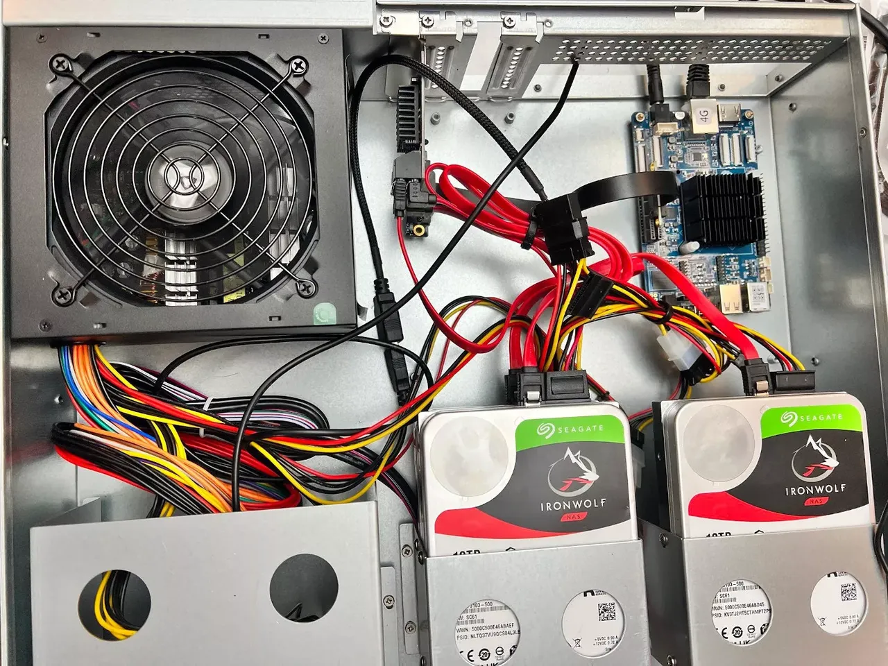
I purchased four Seagate IronWolf 10TB drives. These are spinning metal drives not fancy NVME drives. NVME is too cost prohibitive and would ultimately not be performative; e.g. the bottleneck would be the ROCKPro64.
One of the four drives turned out to be a dud; there are only three in the above picture. The original goal was have 30TB of RAID5 -- 30TB of storage with 10TB for parity. But, because I did not want to spend much more on this project, I opted to return the broken drive and settle for 20TB of storage with 10TB of parity.
The setup is fairly simple. The 2U case, three 10TB drives, a ROCKPro64 4GB single board computer, and a 450W ATX power supply.
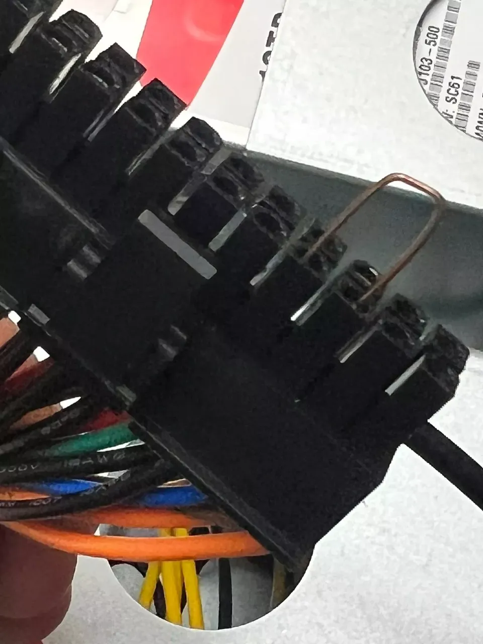
Here's a pro-tip on using a power supply without a motherboard: while holding the power connector with the latching tab towards you, use a paper clip, or in my case, a piece of MIG welding wire, to short out the third and fourth connectors. This probably will void the warranty if something happens to the power supply.
Here is a bit of information on the tech specs of the ROCKPro64.
The drive setup is straight forward. Three drives, running in a RAID5 configuration producing a total of 20TB of usable storage. Setting up software RAID under Linux is simple. I used this as a foundation for setting up software RAID. We are using software RAID because hardware RAID controllers are expensive and have limited support with single board computers. The one that appears to work, is about $600. It is not that I would not be against spending that much on a shiny new controller, it is that I do not feel there would be a noticeable benefit over a pure software solution. I will go into performance characteristics of the software RAID configuration later in this article.
How To Create RAID5 Arrays with mdadm
RAID5 has a requirement of at least three drives. As previously mentioned, this gives you n - 1 drives of storage with one drive's worth of storage for parity. This parity is not stored on the single drive, it is stored across all of the drives but it is equal in total to the size of one drive. There is the assumption that all drives are of equal size.
Get a pretty list of all the available disk:
$ lsblk -o NAME,SIZE,FSTYPE,TYPE,MOUNTPOINT
NAME          SIZE FSTYPE  TYPE  MOUNTPOINT
sda           9.1T         disk
sdb           9.1T         disk
sdc           9.1T         disk
mtdblock0      16M         disk
mmcblk2      58.2G         disk
└─mmcblk2p1  57.6G ext4    part  /
mmcblk2boot0    4M         disk
mmcblk2boot1    4M         disk
You will see we have three, "10TB" drives.
To create a RAID 5 array with the three 9.1T disks, pass them into the mdadm --create command. We will have to specify the device name you wish to create, the RAID level, and the number of devices. We will be naming the device /dev/md0, and include the disks that will build the array:
sudo mdadm --create --verbose /dev/md0 --level=5 --raid-devices=3 /dev/sda /dev/sdb /dev/sdc
This will start to configure the array. mdam uses the recovery process to build the array. This process can and will take some time to complete, but the array can be used during this time. You can monitor the progress of the mirroring by checking the /proc/mdstat file:
$ cat /proc/mdstat
Personalities : [raid6] [raid5] [raid4] [linear] [multipath] [raid0] [raid1] [raid10]
md0 : active raid5 sda[0] sdc[3] sdb[1]
      19532609536 blocks super 1.2 level 5, 512k chunk, algorithm 2 [3/3] [UUU]
      bitmap: 0/73 pages [0KB], 65536KB chunk

unused devices: <none>
For this 20TB to build, it took over 2000 minutes or about a day and half. Once the building is complete, your /proc/mdstat will look similar to the above.
Make a file system on our new array:
$ sudo mkfs.ext4 -F /dev/md0
Make a directory:
$ sudo mkdir -p /mnt/md0
Mount the new array device
$ sudo mount /dev/md0 /mnt/md0
Check to see if the new array is available:
$ df -h -x devtmpfs -x tmpfs
Filesystem      Size  Used Avail Use% Mounted on
/dev/mmcblk2p1   57G  8.7G   48G  16% /
/dev/md0         19T   80K   18T   1% /mnt/md0
Now, let's save our array's configuration:
$ sudo mdadm --detail --scan | sudo tee -a /etc/mdadm/mdadm.conf
Update initramfsso we can use our new array on boot:
$ sudo update-initramfs -u
Add our device to fstab:
$ echo '/dev/md0 /mnt/md0 ext4 defaults,nofail,discard 0 0' | sudo tee -a /etc/fstab
From some of the other documentation, there is a note that dumping the configuration to /etc/mdadm/mdadm.conf before the array is completely built, could result in the number of spare devices not being set correctly. This is what mdadm.conf looks like:
# mdadm.conf
#
# !NB! Run update-initramfs -u after updating this file.
# !NB! This will ensure that initramfs has an uptodate copy.
#
# Please refer to mdadm.conf(5) for information about this file.
#

# by default (built-in), scan all partitions (/proc/partitions) and all
# containers for MD superblocks. alternatively, specify devices to scan, using
# wildcards if desired.
#DEVICE partitions containers

# automatically tag new arrays as belonging to the local system
HOMEHOST <system>

# instruct the monitoring daemon where to send mail alerts
MAILADDR root

# definitions of existing MD arrays

# This configuration was auto-generated on Thu, 22 Dec 2022 16:46:51 -0500 by mkconf
ARRAY /dev/md0 metadata=1.2 spares=1 name=k8s-controlplane-01:0 UUID=62e3b0e3:3cccb921:0fc8e646:ac33bd0f
Note spares=1 is correct in the case of my set up.
By this point, if you have waited until the array has been successfully built - my 20TB array took about a day and half to complete.
Performance
We now have a shiny, new 20TB of available disk space, but what are the performance characteristics of a 20TB, Software RAID5?
We will be using iozone. Iozone has been around for decades; I first used it while in college and having a rack full of servers was all the rage -- before the creation of utility-scale cloud computing, as well as tiny computers.
Download iozone from iozone.org. Extract and compile:
$ cd iozone3_494/src/current
$ make linux
You will end up with the executable iozone in the src/current directory.
Run iozone:
$ sudo ./iozone -a -b output.xls /mnt/md0
This will both output a lot of numbers as well as take a while to complete. When it is complete, you will have an Excel spreadsheet with the results in output.xls.
At this point, I am going to stop doing a step by step of what I have executing and running. Why, I am going to show some visualizations and analyses of our results. My steps will be roughly:
- Break out each block of metrics into its own csv file; for example, the first block found in
output.xlswould be saved in its own csv file; let's call itwriter.csv; exclude the headerWriter Reportfrom the csv. Repeat this step for all blocks of reports.
Writer Report
4   8   16  32  64  128 256 512 1024    2048    4096    8192    16384
64  703068  407457  653436  528618  566551
128 504196  306992  433727  962469  498114  757430
256 805021  475990  850282  594276  571198  582035  733527
512 660600  573916  439445  1319250 549959  645703  926116  591299
1024    1102176 1053512 610617  704230  902151  1326505 1011817 1161176 919928
2048    608964  1398145 1329751 822175  1140942 841094  1332432 1308682 1082427 1311879
4096    1066886 1304093 1168634 946820  1467135 881253  1360802 931521  1047309 1018923 1047054
8192    955344  1295186 1329052 1354035 1019915 1192806 1373082 1197294 1053501 866339  1116235 1368760
16384   1471798 1219970 2029709 1957942 2031269 1533341 1570127 1494752 1873291 1370365 1761324 1647601 1761143
32768   0   0   0   0   1948388 1734381 1389173 1315295 1848047 1916465 1944804 1646551 1632605
65536   0   0   0   0   1938246 1933611 1638071 1910004 1885763 1876212 1844374 1721776 1578535
131072  0   0   0   0   1969167 1962833 1921089 1757021 1644607 1780142 1869709 1566404 1356993
262144  0   0   0   0   2025197 2037129 2036955 1747487 1961757 1954913 1934085 1718841 1596327
524288  0   0   0   0   2041397 2080623 2087150 2049656 2007421 2005253 1930617 1876761 1813078
- I used a combination of using Excel (using LibreOffice Calc would work, too) and a Jupyter Notebook. Excel was used to pull out each report's block and then save each to a CSV file; the Notebook contains python code for reading in CSVs, and using
matplotlibto produce visualizations.
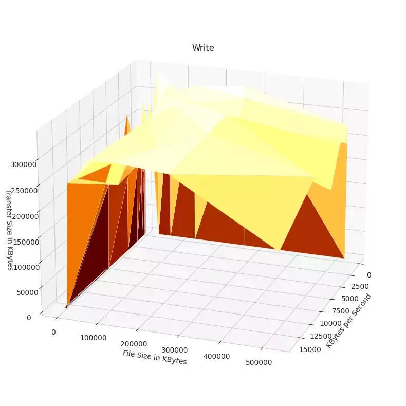
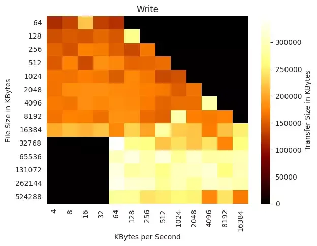
Select Visualizations
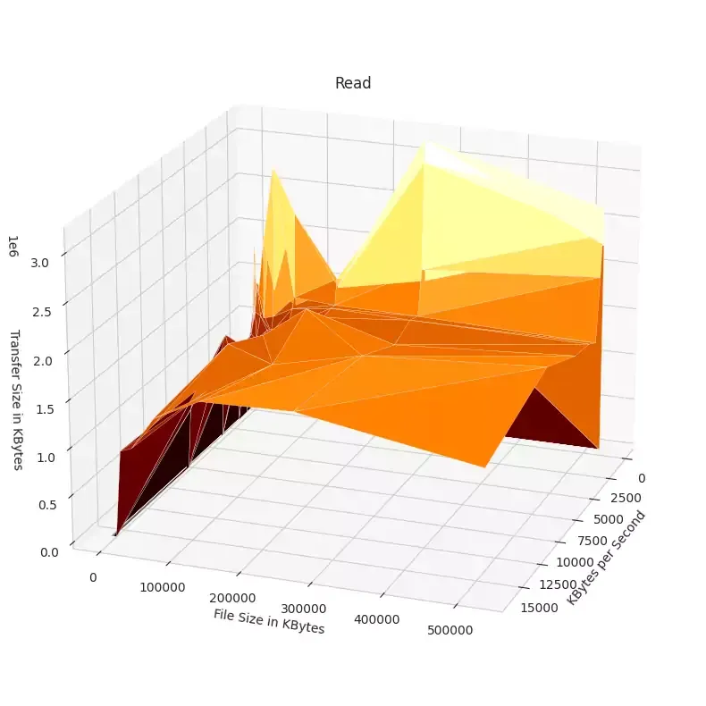
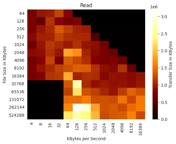
There actually is relatively consistent reads across the file sizes and transfer sizes.