Introduction
Ballistics simulations play a vital role in numerous fields, from defense and military applications to engineering and education. Modeling projectile motion enables the accurate prediction of trajectories for bullets and other objects, informing everything from weapon design and targeting systems to classroom experiments in physics. In a defense context, modeling ballistics is essential for the development and calibration of munitions, the design of effective armor systems, and the analysis of forensic evidence. For engineers, understanding the dynamics of projectiles assists in the optimization of launch mechanisms and safety systems. Educators also use ballistics simulations to illustrate physics concepts such as forces, motion, and energy dissipation.
With Python becoming a ubiquitous language for scientific computing, simulating bullet trajectories in Python presents several advantages. The language boasts a rich ecosystem of scientific libraries and is accessible to both professionals and students. Furthermore, Python’s readability and wide adoption ease collaboration and reproducibility, making it an ideal choice for complex simulation tasks.
This article introduces a Python-based exterior ballistics simulation, leveraging TensorFlow and TensorFlow Probability to numerically solve the equations of motion that govern a bullet's flight. The simulation incorporates a physics-based projectile model, parameterized via real-world properties such as mass, caliber, and drag coefficient. The code demonstrates how to configure environmental and projectile-specific parameters, employ a G1 drag model for small-arms ballistics, and integrate with an advanced ordinary differential equation (ODE) solver. Through this approach, users can not only predict trajectories but also explore the sensitivity of projectile behavior to changes in physical and environmental conditions, making it both a practical tool and a powerful educational resource.
Exterior Ballistics: An Overview
Exterior ballistics is the study of a projectile's behavior after it exits the muzzle of a firearm but before it reaches its target. Unlike interior ballistics (which concerns itself with processes inside the barrel, such as powder combustion and projectile acceleration) exterior ballistics focuses on the forces that act on the bullet in free flight. This discipline is crucial in defense and engineering, as it provides the foundation for accurate targeting, weapon design, and forensic analysis of projectile impacts.
The primary forces and principles governing exterior ballistics are gravity, air resistance (drag), and the initial conditions at launch, most notably the launch angle. Gravity acts on the projectile by pulling it downward, causing its path to curve toward the ground, a phenomenon familiar as "bullet drop." Drag arises from the interaction between the projectile and air molecules, slowing it down and altering its trajectory. The drag force depends on factors such as the projectile's shape, size (caliber), velocity, and the density of the surrounding air. The configuration of the launch angle relative to the ground determines the initial direction of flight; small changes in angle can have significant effects on both the range and the height of the trajectory.
In practice, understanding exterior ballistics is indispensable. Military and law enforcement agencies use ballistic simulations to improve marksmanship, design more effective munitions, and reconstruct shooting incidents. Engineers rely on exterior ballistics to optimize projectiles for maximum range or precision, while forensic analysts use ballistic paths to trace bullet origins. In educational contexts, ballistics offers engaging and practical examples of Newtonian physics, providing real-world applications for students to understand concepts such as forces, motion, energy loss, and the complexities of real trajectories versus idealized “no-drag” parabolas.
The Code: The Setup
The CONFIG dictionary is the central location in the code where all critical simulation parameters are defined. This structure allows users to quickly adjust the model to fit various projectiles, environments, and target scenarios.
Here is a breakdown and analysis of the CONFIG dictionary used in the ballistics simulation:
| Parameter | Value | Description |
|---|---|---|
| target_distance_m | 500.0 | Distance from muzzle to target (meters) |
| muzzle_height_m | 1.0 | Height of muzzle above ground level (meters) |
| muzzle_velocity_mps | 920.0 | Projectile speed at muzzle (meters/second) |
| mass_kg | 0.00402 | Projectile mass (kilograms) |
| diameter_m | 0.0057 | Projectile diameter (meters) |
| air_density_kgpm3 | 1.225 | Ambient air density (kg/m³) |
| gravity_mps2 | -9.80665 | Local gravitational acceleration (meters/second²) |
| drag_family | G1 | Drag model used in simulation (e.g., G1) |
Explanation:
-
Projectile Characteristics:
The caliber (diameter), mass, and muzzle velocity specify the physical and performance attributes of the bullet. These values directly affect the range, stability, and drop of the projectile. -
Environmental Conditions:
Air density and gravity are crucial because they influence drag and bullet drop, respectively. Variations here simulate different weather, altitude, or planetary conditions. -
Drag Model (‘G1’):
The drag model dictates how air resistance is calculated. The G1 model is widely used for small arms and captures more realistic aerodynamics than simple drag assumptions. -
Target Parameters:
Target distance defines the shot challenge, while muzzle height impacts the initial vertical position relative to the ground, both of which are key in trajectory calculations.
Why these choices matter:
Each parameter enables simulation under real-world constraints. Adjusting them allows users to explore how environmental or projectile modifications impact performance, leading to better-informed design, operational planning, or educational outcomes. The explicit separation and clarity in CONFIG also promote reproducibility and easier experimentation within the simulation framework.
Modeling drag forces is essential for realistic ballistics simulation, as air resistance significantly influences the flight of a projectile. In this code, two approaches to drag modeling are considered: the ‘G1’ model and a ‘simple’ drag model.
Drag Models: ‘G1’ vs. ‘Simple’
A ‘simple’ drag model often assumes a constant drag coefficient ($C_d$), applying the drag force as:
$$
F_d = \frac{1}{2} \rho v^2 C_d A
$$
where $\rho$ is air density, $v$ is velocity, and $A$ is cross-sectional area. While straightforward, this approach does not account for the way air resistance changes with speed, which is crucial for supersonic projectiles or bullets crossing different airflow regimes.
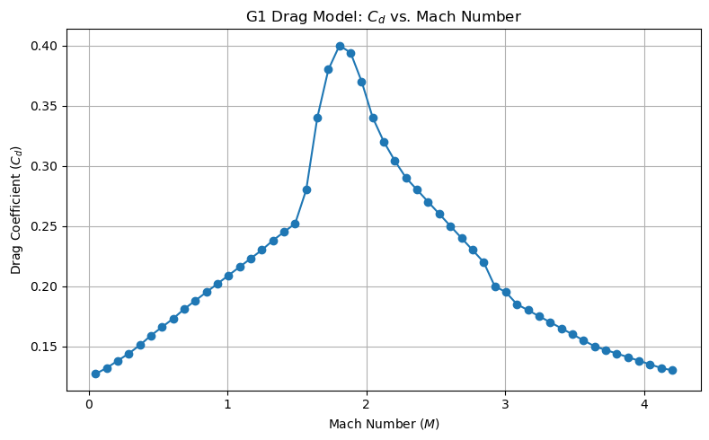
The ‘G1’ model, however, uses a standardized reference projectile and empirically measured coefficients. The G1 drag function provides a table of drag coefficients across a range of Mach numbers ($M$), where $M = \frac{v}{c}$ and $c$ is the local speed of sound. This approach reflects real bullet aerodynamics more accurately than the simple model, making G1 an industry standard for small arms ammunition.
Overview of Drag Coefficients in Ballistics
The drag coefficient ($C_d$) expresses how shape and airflow interact to slow a projectile. For bullets, $C_d$ varies with Mach number due to complex changes in airflow patterns (e.g., transonic shockwaves). Using a fixed $C_d$ (the simple model) ignores these variations and can introduce substantial error, especially for high-velocity rounds.
Why the G1 Model Is Chosen
The G1 model is preferred for small arms because it closely approximates the behavior of typical rifle bullets in the relevant speed range. Manufacturers provide G1 ballistic coefficients, making it easy to parameterize realistic simulations, predict drop, drift, and energy with accuracy, and match real-world data.
Parameterization and Interpolation in Simulation
In the code, the G1 drag is implemented by storing a lookup table of $C_d$ values vs. Mach number. When simulating, the code interpolates between table entries to obtain the appropriate $C_d$ for any given speed. This dynamic, speed-dependent drag calculation enables more precise and physically accurate trajectory modeling.
Let’s visualize a sample G1 drag coefficient curve to illustrate interpolation:
Modeling drag forces is essential for realistic ballistics simulation, as air resistance significantly influences projectile flight. In this code, two approaches to modeling drag are considered: the ‘G1’ model and a ‘simple’ drag model.
Drag Models: ‘G1’ vs. ‘Simple’
A ‘simple’ drag model assumes a constant drag coefficient ($C_d$), applying the drag force as
$
F_d = \frac{1}{2} \rho v^2 C_d A,
$
where $\rho$ is air density, $v$ is velocity, and $A$ is cross-sectional area. While straightforward, this model does not account for the way air resistance changes with speed, an important factor for supersonic projectiles or bullets crossing different airflow regimes.
The ‘G1’ model, by contrast, uses a standardized reference projectile with empirically measured coefficients. The G1 drag function provides a table of drag coefficients across a range of Mach numbers ($M$), where $M = \frac{v}{c}$ and $c$ is the local speed of sound. Unlike the simple model, G1 better reflects real bullet aerodynamics and thus has become the industry standard for small arms ammunition.
Overview of Drag Coefficients in Ballistics
The drag coefficient ($C_d$) describes how shape and airflow interact to slow a projectile. For bullets, $C_d$ varies with Mach number due to changes in airflow patterns (such as transonic shockwaves). Using a fixed $C_d$ (as in the simple model) ignores these variations and may significantly misestimate the trajectory, especially for high-velocity rounds.
Why the G1 Model Is Chosen
The G1 model is simpler for small arms because it approximates the behavior of typical rifle bullets in relevant velocity ranges. Manufacturers publish G1 ballistic coefficients, enabling simulations that accurately predict drop, drift, and retained energy and match real-world results.
Parameterization and Interpolation in Simulation
Within the code, the G1 drag is implemented by storing a lookup table of $C_d$ values versus Mach number. During simulation, the code interpolates between entries in this table to determine the appropriate $C_d$ for any given speed. This allows for speed-dependent drag calculation, giving more precise and physically accurate trajectories.
# ------------------------------------------------------------------------
# 1.  Drag-coefficient functions
# ------------------------------------------------------------------------
def drag_cd_simple(speed):
    mach = speed / 343.0
    cd_sup, cd_sub = 0.295, 0.25
    return tf.where(mach > 1.0,
                    cd_sup,
                    cd_sub + (cd_sup - cd_sub) * mach)

# G1 table  (Mach  →  Cd)
_g1_mach = tf.constant(
   [0.05,0.10,0.15,0.20,0.25,0.30,0.35,0.40,0.45,0.50,0.55,0.60,0.65,0.70,
    0.75,0.80,0.85,0.90,0.95,1.00,1.05,1.10,1.15,1.20,1.25,1.30,1.35,1.40,
    1.45,1.50,1.55,1.60,1.65,1.70,1.75,1.80,1.90,2.00,2.20,2.40,2.60,2.80,
    3.00,3.20,3.40,3.60,3.80,4.00,4.20,4.40,4.60,4.80,5.00], dtype=tf.float64)

_g1_cd   = tf.constant(
   [0.127,0.132,0.138,0.144,0.151,0.159,0.166,0.173,0.181,0.188,0.195,0.202,
    0.209,0.216,0.223,0.230,0.238,0.245,0.252,0.280,0.340,0.380,0.400,0.394,
    0.370,0.340,0.320,0.304,0.290,0.280,0.270,0.260,0.250,0.240,0.230,0.220,
    0.200,0.195,0.185,0.180,0.175,0.170,0.165,0.160,0.155,0.150,0.147,0.144,
    0.141,0.138,0.135,0.132,0.130], dtype=tf.float64)

def drag_cd_g1(speed):
    mach = speed / 343.0
    return tfp.math.interp_regular_1d_grid(
        x                 = mach,
        x_ref_min         = _g1_mach[0],
        x_ref_max         = _g1_mach[-1],
        y_ref             = _g1_cd,
        fill_value        = 'constant_extension')   # <- fixed!

drag_cd = drag_cd_g1 if CONFIG['drag_family'] == 'G1' else drag_cd_simple
Solving projectile motion in exterior ballistics requires integrating a set of coupled, nonlinear ordinary differential equations (ODEs) that account for gravity, drag, and initial conditions. While simple parabolic trajectories can be solved analytically in the absence of air resistance, real-world accuracy necessitates numerical solutions, particularly when drag force is dynamic and velocity-dependent.
This is where TensorFlow Probability’s ODE solvers, such as tfp.math.ode.DormandPrince, excel. The Dormand-Prince method is a member of the Runge-Kutta family of solvers, specifically using an adaptive step size to balance accuracy and computational effort. It’s well-suited for stiff or rapidly changing systems like ballistics, where conditions (e.g., velocity, drag) evolve nonlinearly with time.
Formulation of the Equations of Motion:
The state of the projectile at any time $t$ can be represented by its position and velocity components: $(x, z, v_x, v_z)$. The governing equations are:
$ \frac{dx}{dt} = v_x $
$ \frac{dz}{dt} = v_z $
$ \frac{dv_x}{dt} = - \frac{1}{2}\rho v C_d A \frac{v_x}{m} $
$ \frac{dv_z}{dt} = g - \frac{1}{2}\rho v C_d A \frac{v_z}{m} $
where $\rho$ is air density, $C_d$ is the (interpolated) drag coefficient, $A$ is the cross-sectional area, $g$ is gravity, $m$ is mass, and $v$ is the magnitude of velocity.
Configuring the Solver:
solver = ode.DormandPrince(atol=1e-9, rtol=1e-7)
-
$atol$ (absolute tolerance) and $rtol$ (relative tolerance) define the allowable error in the numerical solution. Lower values lead to higher accuracy but increased computational effort.
-
Tight tolerances are crucial in ballistic calculations, where small integration errors can cause significant deviations in predicted range or impact point, especially over long distances.
The choice of time step is automated by Dormand-Prince’s adaptive approach: larger steps when the solution is smooth, smaller when dynamics change rapidly (e.g., transonic passage). Additionally, users can define the overall solution time grid, enabling granular output for trajectory analysis.
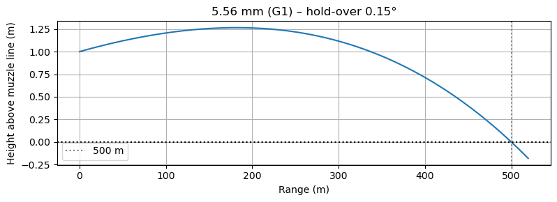
"""
TensorFlow-2 exterior-ballistics demo
• 5.56×45 mm NATO (M855-like)
• G1 drag model with linear interpolation
• Finds launch angle to hit a target at CONFIG['target_distance_m']
"""

# ──────────────────────────────────────────────────────────────────────────
# CONFIG  –– change values here only
# ──────────────────────────────────────────────────────────────────────────
CONFIG = {
    'target_distance_m'  : 500.0,     # metres
    'muzzle_height_m'    : 1.0,       # metres

    # Projectile
    'muzzle_velocity_mps': 920.0,     # m/s
    'mass_kg'            : 0.00402,   # 62 gr
    'diameter_m'         : 0.00570,   # 5.7 mm

    # Environment
    'air_density_kgpm3'  : 1.225,
    'gravity_mps2'       : -9.80665,

    # Drag
    'drag_family'        : 'G1',      # 'G1' or 'simple'

    # Integrator
    'max_time_s'         : 4.0,
    'samples'            : 2000,
}
# ──────────────────────────────────────────────────────────────────────────
# END CONFIG
# ──────────────────────────────────────────────────────────────────────────

import tensorflow as tf
import tensorflow_probability as tfp
import numpy as np
import matplotlib.pyplot as plt

import os


tf.keras.backend.set_floatx('float64')
ode = tfp.math.ode

# ------------------------------------------------------------------------
# Derived constants
# ------------------------------------------------------------------------
g        = tf.constant(CONFIG['gravity_mps2'],      tf.float64)
rho_air  = tf.constant(CONFIG['air_density_kgpm3'], tf.float64)
m        = tf.constant(CONFIG['mass_kg'],           tf.float64)
diam     = tf.constant(CONFIG['diameter_m'],        tf.float64)
A        = 0.25 * np.pi * tf.square(diam)                         # frontal area
v0_muzzle = tf.constant(CONFIG['muzzle_velocity_mps'], tf.float64)

# ------------------------------------------------------------------------
# 1.  Drag-coefficient functions
# ------------------------------------------------------------------------
def drag_cd_simple(speed):
    mach = speed / 343.0
    cd_sup, cd_sub = 0.295, 0.25
    return tf.where(mach > 1.0,
                    cd_sup,
                    cd_sub + (cd_sup - cd_sub) * mach)

# G1 table  (Mach  →  Cd)
_g1_mach = tf.constant(
   [0.05,0.10,0.15,0.20,0.25,0.30,0.35,0.40,0.45,0.50,0.55,0.60,0.65,0.70,
    0.75,0.80,0.85,0.90,0.95,1.00,1.05,1.10,1.15,1.20,1.25,1.30,1.35,1.40,
    1.45,1.50,1.55,1.60,1.65,1.70,1.75,1.80,1.90,2.00,2.20,2.40,2.60,2.80,
    3.00,3.20,3.40,3.60,3.80,4.00,4.20,4.40,4.60,4.80,5.00], dtype=tf.float64)

_g1_cd   = tf.constant(
   [0.127,0.132,0.138,0.144,0.151,0.159,0.166,0.173,0.181,0.188,0.195,0.202,
    0.209,0.216,0.223,0.230,0.238,0.245,0.252,0.280,0.340,0.380,0.400,0.394,
    0.370,0.340,0.320,0.304,0.290,0.280,0.270,0.260,0.250,0.240,0.230,0.220,
    0.200,0.195,0.185,0.180,0.175,0.170,0.165,0.160,0.155,0.150,0.147,0.144,
    0.141,0.138,0.135,0.132,0.130], dtype=tf.float64)

def drag_cd_g1(speed):
    mach = speed / 343.0
    return tfp.math.interp_regular_1d_grid(
        x                 = mach,
        x_ref_min         = _g1_mach[0],
        x_ref_max         = _g1_mach[-1],
        y_ref             = _g1_cd,
        fill_value        = 'constant_extension')   # <- fixed!

drag_cd = drag_cd_g1 if CONFIG['drag_family'] == 'G1' else drag_cd_simple

# ------------------------------------------------------------------------
# 2.  ODE right-hand side  (y = [x, z, vx, vz])
# ------------------------------------------------------------------------
def rhs(t, y):
    x, z, vx, vz = tf.unstack(y)
    v_mag = tf.sqrt(vx*vx + vz*vz) + 1e-9
    Cd    = drag_cd(v_mag)
    Fd    = 0.5 * rho_air * Cd * A * v_mag * v_mag
    ax    = -(Fd / m) * (vx / v_mag)
    az    =  g       - (Fd / m) * (vz / v_mag)
    return tf.stack([vx, vz, ax, az])

solver = ode.DormandPrince(atol=1e-9, rtol=1e-7)

# ------------------------------------------------------------------------
# 3.  Integrate one trajectory for a given launch angle
# ------------------------------------------------------------------------
def shoot(angle_rad):
    vx0 = v0_muzzle * tf.cos(angle_rad)
    vz0 = v0_muzzle * tf.sin(angle_rad)
    y0  = tf.stack([0.0,
                    CONFIG['muzzle_height_m'],
                    vx0, vz0])
    tgrid = tf.linspace(0.0, CONFIG['max_time_s'], CONFIG['samples'])
    sol   = solver.solve(rhs, 0.0, y0, solution_times=tgrid)
    return sol.states.numpy()      # (N,4)

# ------------------------------------------------------------------------
# 4.  Find angle that puts bullet at ground level @ target distance
# ------------------------------------------------------------------------
D = CONFIG['target_distance_m']

def height_at_target(angle):
    traj = shoot(angle)
    x, z = traj[:,0], traj[:,1]
    idx  = np.searchsorted(x, D)
    if idx == 0 or idx >= len(x):      # didn’t reach D
        return 1e3
    x0,x1, z0,z1 = x[idx-1], x[idx], z[idx-1], z[idx]
    return z0 + (z1 - z0)*(D - x0)/(x1 - x0)

low, high = np.deg2rad(-2.0), np.deg2rad(6.0)
for _ in range(40):
    mid = 0.5*(low+high)
    if height_at_target(mid) > 0:
        high = mid
    else:
        low  = mid
angle_solution = 0.5*(low+high)
print(f"Launch angle needed ({CONFIG['drag_family']} drag): "
      f"{np.rad2deg(angle_solution):.3f}°")

# ------------------------------------------------------------------------
# 5.  Final trajectory & plot
# ------------------------------------------------------------------------
traj = shoot(angle_solution)
x, z = traj[:,0], traj[:,1]
mask = x <= D + 20
x, z = x[mask], z[mask]

plt.figure(figsize=(8,3))
plt.plot(x, z)
plt.axvline(D, ls=':', color='gray', label=f"{D:.0f} m")
plt.axhline(0, ls=':', color='k')
plt.title(f"5.56 mm (G1) – hold-over {np.rad2deg(angle_solution):.2f}°")
plt.xlabel("Range (m)")
plt.ylabel("Height above muzzle line (m)")
plt.grid(True)
plt.legend()
plt.tight_layout()
plt.show()
Efficient simulation of exterior ballistics involves careful consideration of runtime, memory usage, and numerical stability. Solving ODEs at every trajectory step can be computationally intensive, especially with high accuracy requirements and long-distance simulations. Memory consumption largely depends on the number of trajectory points stored and the complexity of the drag model interpolation. Numerical stability is paramount; ill-chosen solver parameters might result in nonphysical results or failed integrations. Unfortunately, tensorflow_probability's ODE solver does not take advantage of any GPUs present on the host, it will, instead, utilize CPU. This is a distinct disadvantage compared to torchdiffeq or jax's ode, which can leverage GPU acceleration for ODE solving.
There is an inherent trade-off between accuracy and performance in ODE solving. Tighter solver tolerances (lower $atol$ and $rtol$ values) yield more precise trajectories but at the cost of increased computation time. Conversely, relaxing these tolerances speeds up simulations but may introduce integration errors, which could impact the reliability of performance predictions.
Another trade-off is the use of G1 drag model. The shape of the G1 bullet is not a perfect match for all projectiles, and the drag coefficients are based on empirical data. This means that while the G1 model provides a good approximation for many bullets, it may not be accurate for all types of ammunition. Particularly more modern boat-tail designs with shallow ogive. The simple drag model, while computationally less expensive, does not account for the complexities of real-world drag forces and can lead to significant errors in trajectory predictions.
Conclusion
We have explored the principles of exterior ballistics and demonstrated how to simulate bullet trajectories using Python and TensorFlow. By leveraging TensorFlow Probability's ODE solvers, we were able to model the complex dynamics of projectile motion, including drag forces and environmental conditions. The simulation framework provided a flexible tool for analyzing the effects of various parameters on bullet trajectories, making it suitable for both practical applications and educational purposes.