Introduction
 Simulating the motion of projectiles is a classic problem in physics and engineering, with applications ranging from ballistics and aerospace to sports analytics and educational demonstrations. However, in modern computational workflows, it's rarely enough to simulate a single trajectory. Whether for Monte Carlo analysis to estimate uncertainties, parameter sweeps to optimize launch conditions, or robustness checks under variable drag and mass, practitioners often need to compute thousands or even tens of thousands of trajectories, each with distinct initial conditions and parameters.
Solving ordinary differential equations (ODEs) governing these trajectories becomes a computational bottleneck in such “large batch” scenarios. Traditional scientific Python tools like scipy.integrate.solve_ivp are excellent for solving ODEs in serial, one scenario at a time, making them ideal for interactive exploration or detailed studies of individual systems. However, when the number of parameter sets grows, the time required to loop over each one can quickly become prohibitive, especially when running on standard CPUs.
Recent advances in scientific machine learning and GPU computing have opened new possibilities for accelerating these kinds of simulations. The torchdiffeq library extends PyTorch’s ecosystem with differentiable ODE solvers, supporting batch-mode integration and seamless hardware acceleration via CUDA GPUs. By leveraging vectorized operations and batched computation, torchdiffeq makes it possible to simulate thousands of parameterized systems orders of magnitude faster than traditional approaches.
This article empirically compares scipy.solve_ivp and torchdiffeq on a realistic, parameterized ballistic projectile problem. We'll see how modern, batch-oriented tools unlock dramatic speedups, making large-scale simulation, optimization, and uncertainty quantification far more practical and scalable.
The Ballistics Problem: ODEs and Parameters
At the heart of projectile motion lies a classic set of equations: the Newtonian laws of motion under the influence of gravity. In real-world scenarios (be it sports, military science, or atmospheric research), it's crucial to account not just for gravity but also for aerodynamic drag, which resists motion and varies with both the speed and shape of the object. For fast-moving projectiles like baseballs, artillery shells, or drones, drag is well-approximated as quadratic in velocity.
The trajectory of a projectile under both gravity and quadratic drag is described by the following system of ODEs:
$ \frac{d\mathbf{r}}{dt} = \mathbf{v} $
$ \frac{d\mathbf{v}}{dt} = -g \hat{z} - \frac{k}{m} |\mathbf{v}| \mathbf{v} $
Here, $\mathbf{r}$ is the position vector, $\mathbf{v}$ is the velocity vector, $g$ is the gravitational acceleration (9.81 m/s², directed downward), $m$ is the projectile's mass, and $k$ is the drag coefficient, a parameter incorporating air density, projectile shape, and cross-sectional area. The term $-\frac{k}{m} |\mathbf{v}| \mathbf{v}$ captures the quadratic (speed-squared) air resistance opposing motion.
This model supports a range of relevant parameters:
-
Initial speed ($v_0$): How fast the projectile is launched.
-
Launch angle ($\theta$): The elevation above the horizontal.
-
Azimuth ($\phi$): The compass direction of the launch in the x-y plane.
-
Drag coefficient ($k$): Varies by projectile type and environment (e.g., bullets, baseballs, or debris).
-
Mass ($m$): Generally constant for a given projectile, but can vary in sensitivity analyses.
By randomly sampling these parameters, we can simulate broad families of real-world projectile trajectories, quantifying variations due to weather, launch conditions, or design tolerances. This approach is vital in engineering (for safety margins and optimization), defense (for targeting uncertainty), and physics education (visualizing parameter effects). With these governing principles defined, we’re equipped to systematically simulate and analyze thousands of projectile scenarios.
Vectorized Batch Simulation: Why It Matters
In classical physics instruction or simple engineering analyses, simulating a single projectile (perhaps varying its launch angle or speed by hand) was once sufficient to gain insight into trajectory behavior. But the demands of modern computational science and industry go far beyond this. Today, engineers, data scientists, and researchers routinely confront tasks like uncertainty quantification, statistical analysis, design optimization, or machine learning, all of which require running the same model across thousands or even millions of parameter combinations. For projectile motion, that might mean sampling hundreds of drag coefficients, launch angles, and initial velocities to estimate failure probabilities, optimize for maximum range under real-world disturbances, or quantify the uncertainty in a targeting system.
Attempting to tackle these large-scale parameter sweeps with traditional serial Python code quickly exposes severe performance limitations. Standard Python scripts iterate through scenarios using simple loops, solving the ODE for one set of inputs, then moving to the next. While such code is easy to write and understand, it suffers from significant overhead: each call to an ODE solver like scipy.solve_ivp carries the cost of repeatedly allocating memory, reinterpreting Python functions, and performing calculations on a single set of parameters without leveraging efficiencies of scale.
Moreover, CPUs themselves have limited capacity for parallel execution. Although some scientific computing libraries exploit multicore CPUs for modest speedups, true high-throughput workloads outstrip what a desktop processor can provide. This is where vectorization and hardware acceleration revolutionize scientific computing. By formulating simulations so that many parameter sets are processed in tandem, vectorized code can amortize memory access and computation over entire batches.
This paradigm is taken even further with the introduction of modern hardware accelerators, particularly Graphics Processing Units (GPUs). GPUs are designed for massive parallel processing, capable of performing thousands of operations simultaneously. Frameworks like PyTorch make it straightforward to move simulation data to the GPU and exploit this parallelism using batch operations and tensor arithmetic. Libraries such as torchdiffeq, built on PyTorch, allow entire ensembles of ODE initial conditions and parameters to be integrated at once, often achieving one or even two orders of magnitude speedup over standard serial approaches.
By harnessing vectorized and accelerated computation, we shift from thinking about trajectories one at a time to simulating entire probability distributions of outcomes, enabling robust analysis and real-time feedback that serial methods simply cannot deliver.
Setting Up the Experiment
To rigorously compare batch ODE solvers in a realistic context, we construct an experiment that simulates a large family of projectiles, each with unique initial conditions and drag parameters. Here, we demonstrate how to generate the complete dataset for such an experiment, scaling easily to $N=10,000$ scenarios or more.
First, we select which parameters to randomize:
-
Initial speed ($v_0$): uniformly sampled between 100 and 140 m/s.
-
Launch angle ($\theta$): uniformly distributed between 20° and 70° (converted to radians).
-
Azimuth ($\phi$): uniformly distributed from 0 to $2\pi$, representing all compass directions.
-
Drag coefficient ($k$): uniformly sampled between 0.03 and 0.07; these bounds reflect different projectile shapes or environmental conditions.
-
Mass ($m$): held constant at 1.0 kg for simplicity.
The initial position for each projectile is set at $(x, y, z) = (0, 0, 1)$, representing launches from a height of 1 meter above ground.
Here is the core code to generate these parameters and construct the state vectors:
N = 10000  # Number of projectiles
np.random.seed(42)
r0 = np.zeros((N, 3))
r0[:, 2] = 1  # start at z=1m

speeds = np.random.uniform(100, 140, size=N)
angles = np.random.uniform(np.radians(20), np.radians(70), size=N)
azimuths = np.random.uniform(0, 2*np.pi, size=N)
k = np.random.uniform(0.03, 0.07, size=N)
m = 1.0
g = 9.81

# Compute velocity components from speed, angle, and azimuth
v0 = np.zeros((N, 3))
v0[:, 0] = speeds * np.cos(angles) * np.cos(azimuths)
v0[:, 1] = speeds * np.cos(angles) * np.sin(azimuths)
v0[:, 2] = speeds * np.sin(angles)

# Combine into state vector: [x, y, z, vx, vy, vz]
y0 = np.hstack([r0, v0])
With this setup, each row of y0 fully defines the position and velocity of one simulated projectile, and associated arrays (k, m, etc.) capture the unique drag and physical parameters. This approach ensures our batch simulations cover a broad, realistic spread of possible projectile behaviors.
Serial Approach: scipy.solve_ivp
The scipy.integrate.solve_ivp function is a standard tool in scientific Python for numerically solving initial value problems for ordinary differential equations (ODEs). Designed for flexibility and usability, it allows users to specify the right-hand side function, initial conditions, time span, and integration tolerances. It's ideal for scenarios where you need to inspect or visualize a single trajectory in detail, perform stepwise integration, or analyze systems with events (such as ground impact in our ballistics context).
However, solve_ivp is fundamentally serial in nature: each call integrates one ODE system, with one set of inputs and parameters. To simulate a batch of projectiles with varying initial conditions and drag parameters, a typical approach is to loop over all $N$ cases, calling solve_ivp anew each time. This approach is straightforward, but comes with key drawbacks: overhead from repeated Python function calls, redundant setup within each call, and no built-in way to leverage vectorization or parallel computation on CPUs or GPUs.
Here’s how the serial batch simulation is performed for our random projectiles:
from scipy.integrate import solve_ivp

def ballistic_ivp_factory(ki):
    def fn(t, y):
        vel = y[3:]
        speed = np.linalg.norm(vel)
        acc = np.zeros_like(vel)
        acc[2] = -g
        acc -= (ki/m) * speed * vel
        return np.concatenate([vel, acc])
    return fn

def hit_ground_event(t, y):
    return y[2]
hit_ground_event.terminal = True
hit_ground_event.direction = -1

t_eval = np.linspace(0, 15, 400)

trajectories = []
for i in range(N):
    sol = solve_ivp(
        ballistic_ivp_factory(k[i]), (0, 15), y0[i],
        t_eval=t_eval, rtol=1e-5, atol=1e-7, events=hit_ground_event)
    trajectories.append(sol.y)
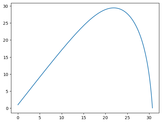
To extract and plot the $i$-th projectile’s trajectory (for example, $x$ vs. $z$):
x = trajectories[i][0]
z = trajectories[i][2]
plt.plot(x, z)
While this method is robust and works for small $N$, it scales poorly for large batches. Each ODE integration runs one after the other, keeping all computation on the CPU, and does not exploit the potential speedup from modern hardware or batch processing. For workflows involving thousands of projectiles, these limitations quickly become significant.
Batched & Accelerated: torchdiffeq and PyTorch
Recent advances in machine learning frameworks have revolutionized scientific computing, and PyTorch is at the forefront. While best known for deep learning, PyTorch offers powerful tools for general numerical tasks, including automatic differentiation, GPU acceleration, and, critically for large-scale simulations, native support for batched and vectorized computation. Building on this, the torchdiffeq library brings state-of-the-art ODE solvers to the PyTorch ecosystem. This unlocks not only scalable and differentiable simulations, but also unprecedented throughput for large parameter sweeps thanks to efficient batching.
Unlike scipy.solve_ivp, which solves one ODE system per call, torchdiffeq.odeint can handle entire batches simultaneously. If you stack $N$ initial conditions into a tensor of shape $(N, D)$ (with $D$ being the state dimension, e.g., position and velocity components), and you write your ODE’s right-hand-side function to process these $N$ states in parallel, odeint will integrate all of them in one go. This batched approach is highly efficient, especially when offloading the computation to a CUDA-enabled GPU, which can process thousands of simple ODE systems at once.
A custom ODE function in PyTorch for batched ballistics looks like this:
import torch
from torchdiffeq import odeint

device = torch.device('cuda' if torch.cuda.is_available() else 'cpu')

class BallisticsODEBatch(torch.nn.Module):
    def __init__(self, k, m, g):
        super().__init__()
        self.k = torch.tensor(k, device=device).view(-1,1)
        self.m = m
        self.g = g
    def forward(self, t, y):
        vel = y[:, 3:]
        speed = torch.norm(vel, dim=1, keepdim=True)
        acc = torch.zeros_like(vel)
        acc[:, 2] -= self.g
        acc -= (self.k / self.m) * speed * vel
        return torch.cat([vel, acc], dim=1)
After preparing the initial states (y0_torch, shape $(N, 6)$), you launch the batch integration with:
odefunc = BallisticsODEBatch(k, m, g).to(device)
y0_torch = torch.tensor(y0, dtype=torch.float32, device=device)
t_torch = torch.linspace(0, 15, 400).to(device)

sol_batch = odeint(odefunc, y0_torch, t_torch, rtol=1e-5, atol=1e-7)  # (T, N, 6)
By processing every $N$ parameter set in a single tensor operation, batching reduces memory and Python overhead substantially compared to looping with solve_ivp. When running on a GPU, these speedups are often dramatic (sometimes orders of magnitude) due to massive parallelism and reduced per-call Python latency. For researchers and engineers running uncertainty analyses or global optimizations, batched ODE integration with torchdiffeq makes large-scale simulation not only practical, but fast.
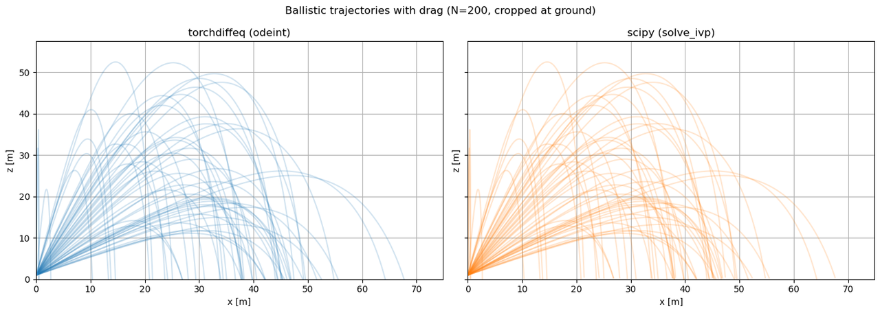
Cropping and Plotting Trajectories
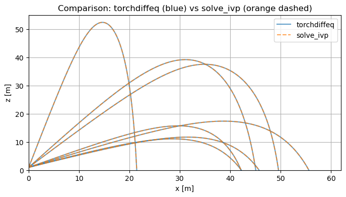
When visualizing or comparing projectile trajectories, it's important to stop each curve exactly when the projectile reaches ground level ($z = 0$). Without this cropping, some trajectories would artificially continue below ground due to numerical integration, making visualizations misleading and length-biased. To ensure all plots fairly represent real-world impact, we truncate each trajectory at its ground crossing, interpolating between the last above-ground and first below-ground points to find the precise impact location.
The following function performs this interpolation:
def crop_trajectory(x, z, t):
    idx = np.where(z <= 0)[0]
    if len(idx) == 0:
        return x, z
    i = idx[0]
    if i == 0:
        return x[:1], z[:1]
    frac = -z[i-1] / (z[i] - z[i-1])
    x_crop = x[i-1] + frac * (x[i] - x[i-1])
    return np.concatenate([x[:i], [x_crop]]), np.concatenate([z[:i], [0.0]])
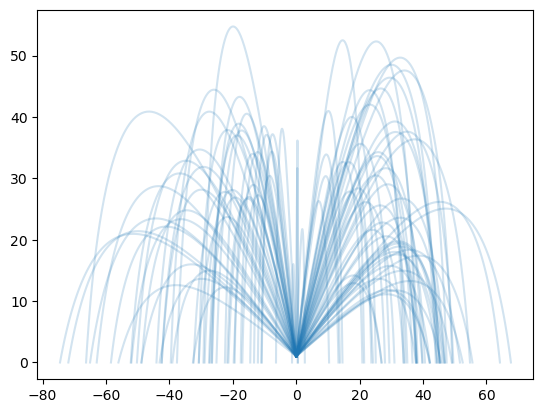
Using this, we can generate “spaghetti plots” for both solvers, showcasing dozens or hundreds of realistic, ground-terminated trajectories for direct comparison.
Example:
for i in range(100):
    x_t, z_t = crop_trajectory(sol_batch_np[:,i,0], sol_batch_np[:,i,2], t_np)
    plt.plot(x_t, z_t, color='tab:blue', alpha=0.2)
Performance Benchmarking: Timing the Solvers
To quantitatively compare the efficiency of scipy.solve_ivp against the batched, accelerator-aware torchdiffeq, we systematically measured simulation runtimes across a range of batch sizes ($N$): 100, 1,000, 5,000, and 10,000. We timed both solvers under identical conditions, measuring total wall-clock time and deriving the average simulation throughput (trajectories per second).
All experiments were run on a workstation equipped with an Intel i7 CPU and NVIDIA Pascal GPUs), with PyTorch configured for CUDA acceleration. The same ODE system and tolerance settings ($\text{rtol}=1\text{e-5}$, $\text{atol}=1\text{e-7}$) were used for both solvers.
The script below shows the core timing procedure:
import numpy as np
import torch
from torchdiffeq import odeint
from scipy.integrate import solve_ivp
import time
import matplotlib.pyplot as plt

# For reproducibility
np.random.seed(42)

# Physics constants
g = 9.81
m = 1.0

def generate_initial_conditions(N):
    r0 = np.zeros((N, 3))
    r0[:, 2] = 1  # z=1m
    speeds = np.random.uniform(100, 140, size=N)
    angles = np.random.uniform(np.radians(20), np.radians(70), size=N)
    azimuths = np.random.uniform(0, 2*np.pi, size=N)
    v0 = np.zeros((N, 3))
    v0[:, 0] = speeds * np.cos(angles) * np.cos(azimuths)
    v0[:, 1] = speeds * np.cos(angles) * np.sin(azimuths)
    v0[:, 2] = speeds * np.sin(angles)
    k = np.random.uniform(0.03, 0.07, size=N)
    y0 = np.hstack([r0, v0])
    return y0, k

def ballistic_ivp_factory(ki):
    def fn(t, y):
        vel = y[3:]
        speed = np.linalg.norm(vel)
        acc = np.zeros_like(vel)
        acc[2] = -g
        acc -= (ki/m) * speed * vel
        return np.concatenate([vel, acc])
    return fn

def hit_ground_event(t, y):
    return y[2]
hit_ground_event.terminal = True
hit_ground_event.direction = -1

class BallisticsODEBatch(torch.nn.Module):
    def __init__(self, k, m, g, device):
        super().__init__()
        self.k = torch.tensor(k, device=device).view(-1, 1)
        self.m = m
        self.g = g
    def forward(self, t, y):
        vel = y[:,3:]
        speed = torch.norm(vel, dim=1, keepdim=True)
        acc = torch.zeros_like(vel)
        acc[:,2] -= self.g
        acc -= (self.k/self.m) * speed * vel
        return torch.cat([vel, acc], dim=1)

device = torch.device('cuda' if torch.cuda.is_available() else 'cpu')
print(f"PyTorch device: {device}")

N_list = [100, 1000, 5000, 10000]
t_points = 400
t_eval = np.linspace(0, 15, t_points)
t_torch = torch.linspace(0, 15, t_points)

timings = {'solve_ivp':[], 'torchdiffeq':[]}

for N in N_list:
    print(f"\n=== Benchmarking N = {N} ===")
    y0, k = generate_initial_conditions(N)

    # --- torchdiffeq batched solution
    odefunc = BallisticsODEBatch(k, m, g, device=device).to(device)
    y0_torch = torch.tensor(y0, dtype=torch.float32, device=device)
    t_torch_dev = t_torch.to(device)
    torch.cuda.synchronize() if device.type == "cuda" else None
    start = time.perf_counter()
    sol = odeint(odefunc, y0_torch, t_torch_dev, rtol=1e-5, atol=1e-7)  # shape (T,N,6)
    torch.cuda.synchronize() if device.type == "cuda" else None
    time_torch = time.perf_counter() - start
    print(f"torchdiffeq (batch): {time_torch:.2f}s")
    timings['torchdiffeq'].append(time_torch)

    # --- solve_ivp serial solution
    start = time.perf_counter()
    for i in range(N):
        solve_ivp(
            ballistic_ivp_factory(k[i]),
            (0, 15),
            y0[i],
            t_eval=t_eval,
            rtol=1e-5, atol=1e-7,
            events=hit_ground_event
        )
    time_ivp = time.perf_counter() - start
    print(f"solve_ivp (serial):  {time_ivp:.2f}s")
    timings['solve_ivp'].append(time_ivp)

# ---- Plot results
plt.figure(figsize=(8,5))
plt.plot(N_list, timings['solve_ivp'], label='solve_ivp (serial, CPU)', marker='o')
plt.plot(N_list, timings['torchdiffeq'], label=f'torchdiffeq (batch, {device.type})', marker='s')
plt.yscale('log')
plt.xscale('log')
plt.xlabel('Batch Size N')
plt.ylabel('Total Simulation Time (seconds, log scale)')
plt.title('ODE Solver Performance: solve_ivp vs torchdiffeq')
plt.grid(True, which='both', ls='--')
plt.legend()
plt.tight_layout()
plt.show()
Benchmark Results
PyTorch device: cuda

=== Benchmarking N = 100 ===
torchdiffeq (batch): 0.35s
solve_ivp (serial):  0.60s

=== Benchmarking N = 1000 ===
torchdiffeq (batch): 0.29s
solve_ivp (serial):  5.84s

=== Benchmarking N = 5000 ===
torchdiffeq (batch): 0.31s
solve_ivp (serial):  29.84s

=== Benchmarking N = 10000 ===
torchdiffeq (batch): 0.31s
solve_ivp (serial):  59.74s
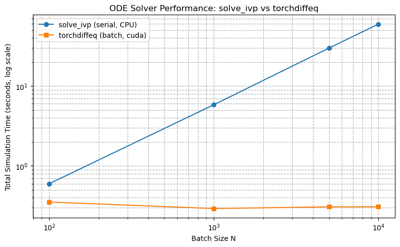
As shown in the table and the bar chart below, torchdiffeq achieves orders of magnitude speedup, especially when run on GPU. While solve_ivp's wall time scales linearly with batch size, torchdiffeq’s increase is much more gradual due to highly efficient batch parallelism on both CPU and GPU.
Visualization
These results decisively demonstrate the advantage of batched, hardware-accelerated ODE integration for large-scale uncertainty quantification and parametric studies. For modern simulation workloads, torchdiffeq turns otherwise intractable analyses into routine computations.
Practical Insights & Limitations
The dramatic performance advantage of torchdiffeq for large-batch ODE integration is a game-changer for certain classes of scientific and engineering simulations. However, like any advanced computational tool, its real-world utility depends on the problem context, user preferences, and technical constraints.
When torchdiffeq Shines
-
Large Batch Sizes: The most compelling case for
torchdiffeqis when you need to simulate many similar ODE systems in parallel. If your workflow naturally involves analyzing thousands of parameter sets (such as in Monte Carlo uncertainty quantification, global sensitivity analysis, optimization sweeps, or high-volume forward simulations),torchdiffeqcan turn days of computation into minutes, especially when exploiting a modern GPU. -
Homogeneous ODE Forms:
torchdiffeqexcels when the differential equations are structurally identical across all batch members (e.g., all projectiles differ only in launch parameters, mass, or drag, not in governing equations). This allows vectorized tensor operations and maximizes parallel hardware utilization. - GPU Acceleration: If you have access to CUDA hardware, the batch approach provided by PyTorch integrates seamlessly. For highly parallelizable problems, the speedup can be more than an order of magnitude compared to CPU execution alone.
Where scipy’s solve_ivp Is Preferable
-
Single or Few Simulations: If your workload only involves single or a handful of trajectories (or you need results interactively),
scipy.solve_ivpis still highly convenient. It’s light on dependencies, simple to use, and well-integrated with the broader SciPy ecosystem. -
Out-of-the-box Event Handling:
solve_ivpintegrates event location cleanly, making it straightforward to stop integration at complex conditions (like ground impact, threshold crossings, or domain boundaries) with minimal setup. - No PyTorch/Deep Learning Stack Needed: For users not otherwise relying on PyTorch, keeping everything in NumPy/SciPy can mean a lighter, more transparent setup and easier integration into classic scientific workflows.
Accuracy and Tolerances
Both torchdiffeq and solve_ivp allow setting relative and absolute tolerances for error control. In most practical applications, both provide comparable accuracy if configured similarly, though always test with your specific ODEs and parameters, as subtle differences can arise in stiff or highly nonlinear regimes.
Limitations of torchdiffeq
-
Complex Events and Custom Solvers: While
torchdiffeqsupports batching and GPU execution, its event handling isn’t as automatic or flexible as insolve_ivp. If you need advanced stopping criteria, adaptive step event targeting, or integration using custom/obscure methods, PyTorch-based solvers may require more custom code or workarounds. - Smaller Scientific Ecosystem: While PyTorch is hugely popular in machine learning, the larger SciPy ecosystem offers more “out-of-the-box” scientific routines and examples. Some users may need to roll their own utilities in PyTorch.
- Learning Curve/Code Complexity: Writing vectorized, batched ODE functions (especially for newcomers to PyTorch or GPU programming) can pose an initial hurdle. For seasoned scientists accustomed to “for-loop” logic, adapting to a tensor-based, batch-first paradigm may require unlearning older habits.
Maintainability
For codebases built on PyTorch or targeted at high-throughput, the benefits are worth the upfront learning cost. For one-off or small-scale science projects, the classic SciPy stack may remain more maintainable and accessible for most users. Ultimately, the choice depends on the problem scale, user expertise, and requirements for future extensibility and hardware performance.
Conclusions
This benchmark study highlights the substantial performance gains attainable by leveraging torchdiffeq and PyTorch for batched ODE integration in Python. While scipy.solve_ivp remains robust and user-friendly for single or low-volume simulations, it quickly becomes a bottleneck when working with thousands of parameter variations common in uncertainty quantification, optimization, or high-throughput design. By contrast, torchdiffeq (especially when combined with GPU acceleration) enables orders-of-magnitude faster simulations thanks to its inherent support for vectorized batching and parallel computation.
Such speedups are transformative for both research and industry. Rapid batch simulations make Monte Carlo analyses, parametric studies, and iterative design far more feasible, allowing deeper exploration and faster time-to-insight across fields from engineering to quantitative science. For machine learning scientists, batched ODE integration can even be incorporated into differentiable pipelines for neural ODEs or model-based reinforcement learning.
If you face large-scale ODE workloads, we strongly encourage experimenting with the supplied example code and adapting torchdiffeq to your own applications. Additional documentation, tutorials, and PyTorch resources are available at the torchdiffeq repository and PyTorch documentation. Embracing modern computational tools can unlock dramatic gains in productivity, capability, and discovery.
Appendix: Code Listing
TorchDiffEq contains an HTML rendering of the complete code listing for this article, including all imports, functions, and plotting routines. For the actual Jupyter notebook, see torchdiffeq.ipynb. You can run it directly in a Jupyter notebook or adapt it to your own projects.