Pattern Recognition as Applied to Peer-to-Peer Lending
The purpose of this article is multi-faceted: 1) to give an overview of what pattern recognition and machine learning are; and 2) the uses of machine learning in the context of and as applied to peer-to-peer lending. This article starts out broad and meanders a bit until it gets into the topic referenced in the title.
Pattern recognition algorithms, as their name suggests, is the recognition of_ patterns_, in data. That is, given a set of inputs (often called features), can an output (sometimes called labels) be inferred? If that seems a bit foreign, well, it should not be. Humans use our own pattern recognitions all the time. When you see a physical book, how do know it’s a book? Maybe you recognize features of the object, it is rectangular, appears to be made of many sheets of paper, there are words on at least two of the larger flat surfaces. Maybe it is a book!
It is likely that someone told you, at one point in your life, that that object in front of you or maybe you were holding it, is a book. This may have happened a few times, and then, all of a sudden, you were able to recognize books. It is very likely that this happened at such a young age, that you do not even remember this first recognition happening. Before going any further, let’s take a detour to explain the other side of this post: peer to peer lending. If you are bit lost, and want to know a bit more about lending, reading the post on the Geography of Social Lending first, then come back to this piece.
Social Lending. When a potential borrower uses one of these systems, and says I would like to obtain a loan, the person enters from identifying information, and from a credit bureau or two, information is pulled into the respective platform. There is a lot of information that is used to determine 1) whether or not a person has a solid enough credit history to take out a loan; and 2) assuming they qualify for a loan, what interest rate should they receive on the loan. All of the peer-to-peer lending platforms have their own proprietary methods for arriving upon the interest rate and usually a proprietary external or resulting risk metric, in the case of Prosper Lending, the source of the data that this article will be using, this risk metric is a letter score of AA to E in addition to HR (which I usually read as high risk).
Many of the features that go into determining this risk metric are actually available. There are roughly 400 different features that are available via Prosper Lending’s platform. Everything from the percent of available credit on an individual’s credit cards, how long has the individual had credit cards, whether the individual has a mortgage, does the individual have any wage garnishments, and the list goes on. Similar to the features that allow a person to identify that a book is a book and not a baseball cap, using the features of an individual’s credit profile, it is possible to get a sense of whether the person will fail to repay the loan. With the availability of loan data from peer-to-peer platforms, there have been a number of competitions to see who can get the most accurate predictions on whether loans will go bad.
If you have been able to follow along so far, great! I fear, however, that I may lose some of you with the following nerd-stuff.
Mathematicians, computer scientists, statisticians, cognitive experts and many in between have developed a fascinating array of algorithms that fall into the category of machine learning. They have fancy names like Support Vector Machines, Ridge and Lasso Regression, Decision Trees, Extra Forest, Random Forests, Gradient Boost, and many others. There are a couple broad groups of problem spaces in machine learning: classification and regression. Classification is pretty much inline with the non-machine-learning definition of the word, which bucket does this thing belong in? With regression, the objective is generally trying to identify a quantity on a continuous spectrum. An example could be, given a person’s gender, height, weight, and maybe a geographic categorization, how much alcohol is this person likely to consume in a given year?
Let’s a take look at regression, first, before looking into classification.
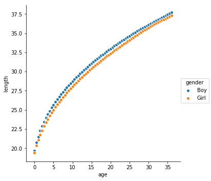
The basic idea behind any of these regression algorithms is to effectively fit a line to a series of points. When you have three or more dimensions in your data, you end up with planes and hyperplanes, but for let’s keep it in simple 2D space for the moment. In a simple example, if you have a plot of points on a graph, let’s say that the Y axis is represents children’s’ height, and the _X _axis represents age in months and you have measurements until the children were age 3 years. For the sake of example date, let’s include the children’s gender (as assigned at birth).
Looking at the graph to the right, there’s a few things you might be able to say. Boys, on average, will be slightly longer than girls of the same age.
What if you had some other data, and it was just age of boys, but you did not have length information on this same set of children?
If you have had a bit of algebra, you might think that there is maybe an equation of a line somewhere in these data. You might think back to y-intercepts _and _slopes of lines. If you thought of this, you just stumbled upon what amounts to 2-dimensional linear regression. As an aside, knowing that the data are of boys is simply filtering out the girls from the data, and that variable, categorical in this case, is not necessary for the following. Remember, that the equation of a line, in slope-intercept form, is y = mx + b.
Using statistical software, like Python’s sci-kit learn, you can use our existing dataset of ages and lengths, to get a linear equation that approximates these data.
import pandas as pd
import matplotlib.pylab as plt
import seaborn as sns
from sklearn.linear_model import LinearRegression
from sklearn.model_selection import train_test_split
import numpy as np

def gender(x):
    if x == 1:
        return "Boy"
    elif x == 2:
        return "Girl"

df = pd.read_excel("https://www.cdc.gov/growthcharts/data/zscore/zlenageinf.xls")
df.columns = ['sex', 'age', 'z_-2', 'z_1.5', 'z_-1', 'z_-0.5', 'mean', 'z_0.5', 'z_1', 'z_1.5', 'z_2']
boys_df = df[df['sex'] == 1]
girls_df = df[df['sex'] == 2]
#### this isn't necessary beyond helping me keep things straight in my head
boys_girls_df = boys_df.append(girls_df)

boys_girls_df['gender'] = boys_girls_df['sex'].map(gender)
#### demetricify these data
boys_df['length'] = boys_df['mean'] * 0.393701
girls_df['length'] = girls_df['mean'] * 0.393701
boys_girls_df['length'] = boys_girls_df['mean'] * 0.393701

x = boys_df['age'].values.ravel()
y = boys_df['length'].values.ravel()

x_training, x_testing, y_training, y_test = train_test_split(x.reshape(-1,1), y)

clf = LinearRegression()
clf.fit(x_training, y_training)
predicts = clf.predict(x_testing)
plt.scatter(x_training, y_training, color='lightblue')
plt.xlabel("age")
plt.ylabel("length")
plt.plot(x_testing, predicts, color='red')

print(clf.coef_[0], clf.intercept_)

plt.show()
The above bit of python code downloads an Excel file from the Center for Disease Control, and puts the columns and rows from that spreadsheet into a table format that more easily programmatically manipulated. Picking the columns necessary for our X _and _Y, as well as subsetting into boys and girls, and putting some labeling on columns, we end up with things that can be pushed into the linear regression machinery. As an aside, you might have noticed the train_test_split method. Basically, the idea before this method is to subset your available data into something you show an algorithm, and something you withhold from the algorithm until later to see how well the algorithm can predict unseen values. This training set and testing set is important, and will be brought up, again, further into this post.
The above code will also print two values, one is the m in the previously mentioned equation, y = mx + b, and the other is the b in that same equation.
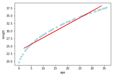
So, our red line has an equation of roughly:
y = 0.438x + 23.399
And if you are thinking that the red line is really not a very great fit for our light blue dots, you would be correct. If you had new data from only 5 month to 30 month old boys, you could approximate the lengths, but if you had data for children outside of these bounds, you would end up approximations that were too long in the case of those very young, and approximations that were too short for those older.
The question now arises, how does one get more closely fitting line to the underlining data__? The answer ends up being, use fancier machines. For the sake simplicity, we will skip over whole groupings of other algorithms and look at one called Gradient Boosting. If you have had more advanced calculus, and the word gradient rings a bell, good. That is the same gradient. Perhaps in a future posting, I’ll jump into explaining gradient boosting, but not now.
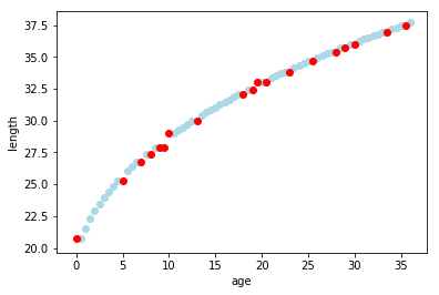
If you swap out the LinearRegression _in above code snippet with _GradientBoostingRegressor, rerun the code, with the print statement commented out, and plt.plot(x_testing, predicts, color=’red’) replaced with plt.scatter(x_testing, predicts, color=’red’), you end up with the graph to the right. As you can see, the red dots, which consist of ages from withheld-from-training age/length pairs, with predicted length, plot neatly within the blue dots of actual data points.
That’s a brief introduction into applying regression to a problem set. Now, what about classifiers?
I tend to think of classifiers as still having dots of data on a graph, and continuing to find a line that fits these data. However, instead of trying to get dots directly on the line, you try to figure out which side of the line the dot belongs to, and then you can say it belongs to category 1, or you can say, it belongs to category 2. In the case of our example infant length and gender data, you age and length as input features to try to categorize the birth gender of a particular child. On the peer-to-peer lending front, this equates into using those 400+ features that included with a loan’s listing to try to get the outcome of success or fail. There is also a probability metric associated with the classification that could be thought of as how close to the dividing line is this prediction?
There are a handful of academic works that look at applying machine learning to the peer-to-peer lending space. The one that seemed to come up the most, as I researched the topic myself for projects during my graduate studies, was a journal article from 2015; Risk Assessment in Social Lending via Random Forests, by Malekipirbazari & Aksakalli. The abstract for that article is as follows:
With the advance of electronic commerce and social platforms, social lending (also known as peer-to-peer lending) has emerged as a viable platform where lenders and borrowers can do business without the help of institutional intermediaries such as banks. Social lending has gained significant momentum recently, with some platforms reaching multi-billion dollar loan circulation in a short amount of time. On the other hand, sustainability and possible widespread adoption of such platforms depend heavily on reliable risk attribution to individual borrowers. For this purpose, we propose a random forest (RF) based classification method for predicting borrower status. Our results on data from the popular social lending platform Lending Club (LC) indicate the RF-based method outperforms the FICO credit scores as well as LC grades in identification of good borrowers__1.
This paper and a few others I have come across use Random Forest, and it seems to be the go to algorithm. Much of the data from peer-to-peer lending platforms are categorical, but some is continuous. Random Forests handle these heterogenous data quite well2.
The general classification idea, when applying machine learning to peer-to-peer lending data, is a binary problem: Do loans succeed in being repaid or do they fail to be repaid?
Risk Assessment in Social Lending via Random Forest is really a great paper. Even though it focuses on the more readily available data from Lending Club, it gives a great job of doing a brief literature review of prior papers that looked into peer-to-peer lending, as well as looking at three different machine learning approaches to the problem. They also highlight that, within Lending Club’s data, simply relying upon the proprietary grade metric, is not necessarily indicative of a good borrower. The concept of good borrower and their identification is, however, the one point that perplexes me. I tend to couch the problem in a different, I want to successfully identify bad borrowers, so as to avoid lending to them. Thinking of the problem space with this notion in mind, also highlights another characteristic of these data: imbalanced classes or categories of final loan state (success or fail). Many classification techniques work best when the classes being evaluated are more or less even in size3. Many canonical classification algorithms have the assumption that the outcome classes of a dataset are balanced4. The data from Prosper lending, after having been mapped into a binary categorization of fail and success, the counts of each outcome show an imbalance across the whole dataset of 75% of the loans were successful, and 25% of loans failed. This imbalance of classes can lead to classifier bias. In my mind, this means that it is easier and more likely that a new, never before seen loan listing will be classified as success by your trained algorithm, then it is to identify loan listings that one should best be avoided.
This imbalance in classes leads us into the general area of preprocessing. If you think of running data through your machine learning algorithm as processing, this is the step before that. The algorithms are pretty sophisticated, but if the data have non-numerical values, for example, the Prosper Rating, the algorithm will not know what to do with these values; these values need to be turned into something numerical. Likewise, with the imbalance of outcome classes, something could be done with this.
Let’s talk more specifically about what preprocessing was done on our Prosper Lending dataset.
If you have an investor account with Prosper, you can freely download two different sets of data. Listing data, and Loan data. Listing data sets contain the borrowers credit profile, the state they reside in, their occupation that has its value originating from a drop down menu or a set of pick-one radio buttons in the user interface, as well as a whole host of other bits of information. Loan data sets contain a sort of snap shot in time as to the current status of a loan, if the loan is still actively being paid off. In the case of loans that have “run their course”, this means that they were either successfully repaid, or they entered into a status of “default” or “charge-off”; both of these statuses for our purposes are considered fails.
We will only be concerned with loans that have either successfully been repaid, or have defaulted or been charged-off. We are not concerned with active, in good standing loans. As an aside, we might be interested in active, in good standing loans, if there was a secondary market to sell loans that are in the process of being repaid. Sadly, Prosper shutdown its secondary market a few years, and as such, once a loan as originated, and the lenders receive notes, those notes are effectively an illiquid asset.
The key piece of information that is missing from these two sets of data is a linkage between the listing from the borrower, and a loan’s final outcome. The field listing_number is noticeably absent from the loan datasets. A linkage between these two datasets is possible by matching the borrower’s state, the borrower’s interest rate on the loan, the date the listing was turned into a loan, and the amount of money of the loan. This will get you nearly all the way to having a correctly set of datasets. But, Prosper does make this linkage data available. More data are available if you inquire and sign a data sharing agreement. The linkage data, however, is in a terribly inconvenient format. It is a 16GB (2GB compressed) comma separated format file that represents every payment and every payment attempt on the Prosper platform from nearly the start of the platform, up to roughly the previous calendar quarter. This enormous file is data rich, and would allow for finer grained analysis of Prosper’s lending and borrowers’ repayment efforts, but the bit that we are interested in the listing_number <-> loan_number pairing that is found in this file. As a side note, I tend to use listing_number (lower case with an underscore), Prosper tends to use ListingNumber (camelcase words); I will go back and forth between the two flavors, but they mean the same thing. I wrote a bit of wrap code that can read in all the zip files in a directory for the listing data and the loans data, and make Prosper’s CamelCase column names into snake_case.
Taking this enormous CSV file, and read it into a Pandas DataFrame, and select the two columns we are interested, ListingNumber and LoanID, then group by two columns:
import pandas as pd
df = pd.read_csv('./LoanLevelMonthly.zip')
loans_listings_df = df.groupby(['LoanID', 'ListingNumber']).size().reset_index()
loans_listings_df.columns = ['loan_number', 'listing_number', 'count']
So, where does one get access these data? You will need to contact Prosper via their help desk and ask for the “Prosper Data License Agreement”. Once you sign and return this agreement to them, within a day or two, you will be sent information on how to download the latest data from the platform.
Then, you will need historical listings and loans data that you will then use the above to link up the listings data and loan outcomes. Assuming you have a Prosper account, and you are already logged in, as I mentioned above, you can just download all the historical data.
At this stage, we are only interested in data on loans that are done. That is, loans that have either been successfully and fully repaid, or loans that have defaulted or has been declared a charge-off. In these data, that means a loan_status of greater 1 and less than 6.
Reading in the listings zip files, you will want to simply read the first (and oldest) file into a Pandas DataFrame, and then read the next oldest, appending that file’s contents to the previously created DataFrame. You will do this with all of the listings zip files. Similarly, read all the loans data into a separate DataFrame, appending the newer loans to the older loans.
After reading in both the listing data and the loan data, we select only the loans with the statuses we want.
loan_df = loan_df[loan_df['loan_status'] > 1]
loan_df = loan_df[loan_df['loan_status'] < 6]
print(loan_df.groupby(['loan_status']).size())
loan_status
2 25244
3 90481
4 361687
dtype: int64
You should have three DataFrames at this point. One DataFrame with the linkings of loan_number to listing_number, one DataFrame containing loans data, and one DataFrame containing listing data.
The only purpose that we link loans to listings is getting loans’ final status, we will want to select out just two columns; the loan_number and the loan_status.
loan_status_df = loan_df[['loan_number', 'loan_status']]
At this point, if we were wanting to do something like figuring out the actual, real rate of return on a loan, that is, the amount of money that the lender ultimately received, you could calculate that value at this stage. It would look something like:
loan_df['actual_return_rate'] = (loan_df['principal_paid'] + loan_df['interest_paid'] + loan_df['service_fees_paid'] - loan_df['amount_borrowed']) / loan_df['amount_borrowed']/(loan_df['term'] / 12)
Note, service_fees_paid is negative, so we just add it to the amount to effective subtract that amount
If we did want to include actual_return_rate, we would include that in the columns we select out (above), but we would need to remember to remove actual_return_rate later, when we are attempting to classifier listings as it would effectively spike our results. Likewise, if we were using a regressor to try to predict the actual_return_rate, you would want to remove loan_status from the mix.
But for now, we will only be concerned with looking at predicting a loan’s outcome solely on what was in the listing for that loan. Back to our three DataFrames.
Start by merging loan_status_df to loans_listings_df.
loans_with_listing_numbers_df = loan_status_df.merge(loans_listings_df,on=['loan_number'])
This will do an inner join on the two DataFrames, and truncate off loans that are too new compared to the loans <–> listings linkage data.
Similarly for the listing data, we merge listing_df with the newly created loans_with_listing_numbers_df
complete_df = loans_with_listing_numbers_df.merge(listing_df,on=['listing_number'])
At this point, you will have a DataFrame that contains hundreds of thousands of rows of heterogeneous data. Some dates, some categorical (e.g. prosper scores, credit score range bins, and so forth), as well as continuous values (usually something dealing with a percent or a dollar amount).
There are also columns that you want to exclude or remove completely because they are present in these historic data but not present in listing data that are obtained via Prosper’s API for active listings. We will filter, remove or otherwise transfer the DataFrame into something is slightly more usable.
def remap_bool(x):
    if x == False:
        return -1
    elif x == 'False':
        return -1
    elif x is None:
        return -1
    elif x == True:
        return 1
    elif x == 'True':
        return 1
    elif x == '0':
        return -1

def to_unixtime(d):
    return time.mktime(d.timetuple())

def to_unixtime_str(d):
    if str(d) == 'nan':
        return  to_unixtime(parser.parse('2006-09-01'))

    return to_unixtime(parser.parse(d))

def remap_str_nan(x):
    return str(x)

def remap_loan_status(x):
    if x == 4:
        return 1
    else:
        return -1

df = complete_df.copy()
df['loan_status'] = df['loan_status'].map(remap_loan_status)
df['has_mortgage'] = df['is_homeowner'].map(remap_bool)
df['first_recorded_credit_line'] = df['first_recorded_credit_line'].map(to_unixtime_str)
df['scorex'] = df['scorex'].map(remap_str_nan)
df['partial_funding_indicator'] = df['partial_funding_indicator'].map(remap_bool)
df['income_verifiable'] = df['income_verifiable'].map(remap_bool)
df['scorex_change'] = df['scorex_change'].map(remap_str_nan)
df['occupation'] = df['occupation'].map(remap_str_nan)
df['fico_score'] = df['fico_score'].map(remap_str_nan)

df = df.drop(['channel_code', 'group_indicator', 'orig_date', 'borrower_city', 'loan_number', 'loan_origination_date', 'listing_creation_date', 'tu_fico_range', 'tu_fico_date', 'oldest_trade_open_date', 'borrower_metropolitan_area', 'credit_pull_date', 'last_updated_date', 'listing_end_date', 'listing_start_date', 'whole_loan_end_date', 'whole_loan_start_date', 'prior_prosper_loans61dpd', 'member_key', 'group_name', 'listing_status_reason', 'Unnamed: 0', 'actual_return_rate', 'investment_type_description', 'is_homeowner', 'listing_status', 'listing_number', 'listing_uid'], axis=1)
We end up with a slightly cleaner, slightly more meaningful (from an algorithm’s perspective) table of data. However, there is still more that can be done to these data. It would be up to you to determine if there were more steps in a pipeline that could be used to make these data more meaningful. Other steps could include removal of outliers via an Isolation Forest5. Dealing with the class imbalance is also something to consider. For our final model that we developed, we used SMOTE6 for oversampling during our training phase. That is, we used SMOTE to take training data and produce synthetic data with balanced classes from a 60% to 75% sampling of the whole data. This leans you legitimate, actual historic data to verify (test) your model with to see how well it predicts what you are interested in predicting.
It should also be mentioned that we one hot encoded our data. We split off the outcome column, and one hot encoded our features. This has the effect of taking the remaining categorical columns, such as borrower_state, and making individual boolean columns for each category in that column (in the case of state, this resulted in something like 52 new columns or something like that).
The model we have actually deployed into a small, real world experiment where, based off the scorings produced with the model, there are actual listings being be automatically invested in, has a pipeline of something like the following:
Linking Dataset -> Cleaning & Translating -> One Hot Encoding -> Anomaly Detection & Removal -> Rescaling data between 0 and 1 -> Oversampling -> Training -> Verification -> Deployment
Getting to the point of having a tuned, deployable model, should actually be the topic of another followup article. The gist of the tuning involves a lot of brute force, grid searching with parameters.
Our final classifier is something like this:
clf_gb = XGBClassifier(n_estimators=639, n_jobs=-1, learning_rate=0.1, gamma=0, subsample=0.8, colsample_bytree=0.8,
 objective= 'binary:logistic', scale_pos_weight=1, max_depth=9, min_child_weight=10, silent=False, verbose=50, verbose_eval=True)
We take the intermediate things, like the min max scaler object, in addition to the classifier itself, and pickle these. Before you get your nerd panties in a twist, we do realize that there are dangers to using pickled objects in python. We’ll assume the risks for now.
These pickled objects then get deployed with a thin wrapper that takes output from Prosper’s API endpoint for listings, and does translation and blows out things to required columns (remember, we one hot encoded things, so, there are a lot of columns to fill out). This then gets run through the model to produce a scoring of success and failure probability.
If you recall, above, that the one thing that we were ultimately concerned with was identifying loans that will most likely fail. Likewise, in that same statement, there is an implicit desire to minimize the number of loans that failed but were classified as being successful during our testing phase. Here is the confusion matrix from our testing phase:
array([[ 8022,  6080],
       [24031, 90805]])
That 6,080 is smallest number in the bunch, we interpret this a good sign. To further possibly address the likelihood of investing in a falsely labeled listing, we also filter on the success probability. Something like exclude listings with a score under 0.85. This still won’t catch truly out of whack listings, but we hope it would help.
Useful Links & Things
- Oversampling: https://beckernick.github.io/oversampling-modeling/
- http://www.ritchieng.com/machine-learning-evaluate-classification-model/
- Measuring classifiers: https://link.springer.com/article/10.1007/s10994-009-5119-5
- What the F-Measure Doesn’t Measure: https://arxiv.org/pdf/1503.06410.pdf
- http://arogozhnikov.github.io/2016/06/24/gradient_boosting_explained.html
- https://www.datasciencecentral.com/profiles/blogs/random-forests-explained-intuitively
- http://faculty.chicagobooth.edu/devin.pope/research/pdf/Website_Prosper.pdf
- https://content.iospress.com/articles/journal-of-intelligent-and-fuzzy-systems/ifs169140
- Evaluating credit risk and loan performance in online Peer-to-Peer (P2P) lending
- https://machinelearningmastery.com/tune-number-size-decision-trees-xgboost-python/
- https://devblogs.nvidia.com/gradient-boosting-decision-trees-xgboost-cuda/