Modeling the Recoil Dynamics of the AR-15 Rifle using Python and Differential Equations
When analyzing the performance of the AR-15 rifle or any firearm, understanding the recoil characteristics is essential. Recoil impacts the ability of shooters to control the rifle, quickly re-acquire targets, and maintain accuracy. In this post, we'll walk through the mathematics and physics behind recoil dynamics and demonstrate how to numerically simulate it using Python.
Understanding Firearm Recoil: A Mechanical Perspective
The Physics of Recoil
Recoil occurs from conservation of momentum: as the bullet and gases accelerate forward through the barrel, the rifle pushes backward against the shooter. To realistically simulate this, we consider the entire shooter-rifle system as a mechanical structure composed of:
- Mass (M): Effective mass of the rifle and shooter.
- Damping (C): Dissipative force (body tissues, rifle buttstock pad).
- Spring (k): The internal buffer spring of the rifle itself.
Modeling as a Mass-Spring-Damper System
We can express this physically as a second-order ordinary differential equation (ODE):
$$ M\frac{d^2x}{dt^2} + C\frac{dx}{dt} + kx = -F_{\text{recoil}}(t) $$
Where:
- $(x(t))$: Rearward displacement.
- $(M)$: Mass of shooter + rifle.
- $(C)$: Damping coefficient (shoulder and body dampening effect).
- $(k)$: Internal rifle-buffer spring stiffness.
- $(F_{\text{recoil}})$: Force during bullet acceleration (short impulse duration).
Converting the Recoil ODE into a Numerical Form
To numerically solve the recoil equation, we'll rewrite it as a set of two first-order equations. Let:
- $(x_1 = x)$
- $(x_2 = \frac{dx}{dt})$
Then:
$$ \frac{dx_1}{dt} = x_2 \ \frac{dx_2}{dt} = \frac{-C x_2 - k x_1 -F_{\text{recoil}}(t)}{M} $$
Recoil Force and Impulse Duration
For the AR-15, recoil force $(F_{\text{recoil}})$ exists briefly while the bullet accelerates. The force can be approximated as the momentum change per impulse duration, i.e.,
$$ F_{\text{recoil}} = \frac{m_{\text{bullet}} v_{\text{bullet}}}{t_{\text{impulse}}} $$
Simulating AR-15 Recoil with Python
Now let's solve the equations numerically. Below are typical AR-15 parameters we will use:
- Rifle & Shooter mass, $(M\ ≈ 5\ \text{kg})$
- Bullet mass, $(m_{bullet}\ ≈ 4\ grams\ ≈ 0.004\ kg)$
- Muzzle velocity, $(v_{bullet}\ ≈ 975\ \text{m/s})$
- Impulse duration, $(t_{\text{impulse}}\ ≈\ 0.5\ ms\ =\ 0.0005\ s)$
- Damping coefficient, $(C ≈ 150\ Ns/m)$ (estimated)
- Internal buffer Spring constant, $(k ≈ 10000\ N/m)$
Python Code Implementation:
import numpy as np
from scipy.integrate import solve_ivp
import matplotlib.pyplot as plt

# AR-15 Parameters
m_bullet = 0.004              # Bullet mass [kg]
v_bullet = 975                # Bullet velocity [m/s]
M = 5.0                       # Effective recoil mass [kg] (rifle + shooter)
C = 150                       # Damping coefficient [N·s/m]
k = 10000                     # Buffer spring constant [N/m]
t_impulse = 0.0005            # Recoil impulse duration [s]

# Compute recoil force
F_recoil = m_bullet * v_bullet / t_impulse

# Define system of equations
def recoil_system(t, y):
    x, v = y
    if t <= t_impulse:
        F = -F_recoil
    else:
        F = 0
    dxdt = v
    dvdt = (-C*v - k*x + F) / M
    return [dxdt, dvdt]

# Initial conditions — rifle initially at rest
init_conditions = [0, 0]

# Time span (0 to 100 ms simulation)
t_span = (0, 0.1)
t_eval = np.linspace(0, 0.1, 5000)

# Numerical Solution
sol = solve_ivp(recoil_system, t_span, init_conditions, t_eval=t_eval)

# Results Extraction
displacement = sol.y[0] * 1000 # convert to mm
velocity = sol.y[1]            # m/s

# Plot Results
plt.figure(figsize=[12, 10])

# Displacement Plot
plt.subplot(211)
plt.plot(sol.t*1000, displacement, label="Displacement (mm)")
plt.axvline(t_impulse*1000, color='r', linestyle="--", label="Impulse End")
plt.title("AR-15 Recoil Displacement with Buffer Spring")
plt.xlabel("Time [ms]")
plt.ylabel("Displacement [mm]")
plt.grid()
plt.legend()

# Velocity Plot
plt.subplot(212)
plt.plot(sol.t*1000, velocity, label="Velocity (m/s)", color="orange")
plt.axvline(t_impulse*1000, color='r', linestyle="--", label="Impulse End")
plt.title("AR-15 Recoil Velocity with Buffer Spring")
plt.xlabel("Time [ms]")
plt.ylabel("Velocity [m/s]")
plt.grid()
plt.legend()

plt.tight_layout()
plt.show()
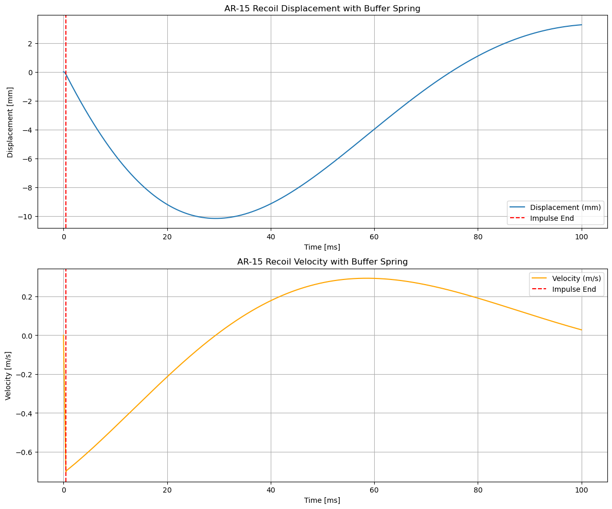
Results: Analyzing the AR-15 Recoil Behavior
In the plots above, the model provides insightful details about how recoil unfolds:
- Rapid initial impulse: The rifle moves backward sharply in the initial half-millisecond recoil impulse stage.
- Buffer spring action: Quickly after the impulse period, the buffer spring engages, significantly reducing velocity and displacement.
- Damping & Recoil absorption: After the initial sharp step, damping forces take effect, dissipating recoil energy, slowing and gradually stopping rifle movement.
This recoil model aligns with how AR-15 rifles mechanically operate in reality: A buffer spring significantly assists in absorbing and dissipating recoil, enhancing accuracy, comfort, and controllability.
Improving the Model Further
While the current simplified model closely reflects reality, future extensions can be considered:
- Nonlinear damping: A real shooter's body provides nonlinear damping. Implementing this would enhance realism.
- Internal Gas Dynamics: Real recoil also involves expanding gases. A more sophisticated model might consider gas forces explicitly.
- Shooter's biomechanics: Accurately modeling human biomechanics as nonlinear springs and dampers could yield even more realistic scenarios.
Final Thoughts
Through numerical simulation with Python and differential equation modeling, we've created an insightful approach to understanding firearm dynamics, in this case the AR-15 platform. Such understanding aids in rifle design improvements, shooter ergonomics, and analysis of recoil management accessories.
Firearm analysts, engineers, and enthusiasts can adapt this flexible simulation method for other firearms, systems with differing parameters, or even entirely different recoil mechanisms.
Through computational modeling like this, the physics underlying firearm recoil becomes uniquely visual and intuitive, enhancing engineering, training, and technique evaluation alike.