Abstract
Machine learning models for ballistic coefficient (BC) correction have demonstrated significant improvements in trajectory prediction accuracy by capturing velocity-dependent drag variations that traditional constant-BC assumptions cannot model. However, deploying such models in field conditions presents challenges: network connectivity requirements, latency constraints, and computational overhead on resource-limited devices. This paper presents a methodology for discretizing continuous ML models into offline lookup tables, specifically addressing the problem of ballistic coefficient corrections across the flight envelope. We construct caliber-specific 5-dimensional lookup tables (BC5D) indexed by bullet weight, base BC, muzzle velocity, instantaneous velocity, and drag model type. Our approach samples the continuous ML function at fixed intervals and relies on piecewise-linear interpolation for queries between sample points. Empirical evaluation demonstrates that this discretization achieves velocity predictions within 5% of the continuous ML model through supersonic and early transonic regimes, with predictable divergence of 10-15% in deep transonic regions (Mach 0.8-1.2) where the underlying physics exhibit pronounced non-linearities. We argue that this accuracy-connectivity trade-off represents a practical compromise for field deployment, analogous to the relationship between analog signals and digital sampling in audio engineering.
1. Introduction and Thesis
The ballistic coefficient (BC) serves as the primary aerodynamic descriptor for projectile flight, encoding the bullet's ability to overcome air resistance into a single dimensionless quantity. Traditionally, manufacturers publish BC values measured under specific conditions (typically referenced to standard atmospheric density at sea level) and these values are treated as constants throughout the trajectory calculation. This simplification, while computationally convenient, ignores a well-documented physical reality: drag characteristics vary substantially with velocity, particularly as projectiles decelerate through transonic regimes where the relationship between Mach number and drag coefficient undergoes rapid, non-linear transitions [1, 2].
Machine learning approaches have emerged as a promising solution to this limitation. By training models on empirical drag data (obtained through Doppler radar tracking, spark range measurements, or computational fluid dynamics simulations) researchers can capture the complex, velocity-dependent nature of aerodynamic drag with greater fidelity than constant-BC assumptions permit [3, 4]. These ML models accept multiple input parameters (bullet geometry, muzzle velocity, current velocity, atmospheric conditions) and output a correction factor that adjusts the published BC to reflect instantaneous flight conditions.
However, ML model deployment introduces practical constraints that conflict with many real-world use cases. Precision shooting applications often occur in environments lacking reliable network connectivity. Mobile devices and embedded systems may lack the computational resources for real-time model inference. Latency requirements for interactive ballistics calculators may preclude round-trip API calls to remote servers. These constraints motivate investigation into methods for deploying ML-derived insights without the ML infrastructure.
Thesis: Continuous machine learning models for ballistic coefficient correction can be effectively discretized into offline lookup tables that preserve the essential predictive improvements while eliminating connectivity and computational dependencies. The discretization introduces a piecewise-linear approximation that follows the general trend of the continuous model but exhibits stair-step behavior at sample boundaries, a trade-off analogous to digital audio sampling, where sufficiently fine discretization renders the steps imperceptible for practical applications.
This paper makes three primary contributions:
- A methodology for constructing caliber-specific 5-dimensional BC correction tables from continuous ML models
- Empirical analysis of approximation fidelity across the velocity envelope, with particular attention to transonic degradation
- A practical deployment architecture enabling offline operation while maintaining compatibility with online systems
2. Background and Related Work
2.1 Ballistic Coefficient Fundamentals
The ballistic coefficient, as formalized by Ingalls and later refined by the Sporting Arms and Ammunition Manufacturers' Institute (SAAMI), relates a projectile's drag characteristics to a standard reference projectile [5]. The G1 and G7 drag models, representing flat-base and boat-tail projectile shapes respectively, define these reference functions. A projectile's BC expresses the ratio of its sectional density to its form factor relative to the standard:
$$BC = \frac{SD}{i} = \frac{m/d^2}{C_D/C_{D_{ref}}}$$
where $m$ is mass, $d$ is diameter, $C_D$ is the projectile's drag coefficient, and $C_{D_{ref}}$ is the reference projectile's drag coefficient at the same Mach number [6].
The critical insight motivating this work is that the form factor $i$ is not constant; it varies with Mach number, particularly in the transonic regime (Mach 0.8-1.2) where shock wave formation and boundary layer interactions produce complex aerodynamic effects [7]. Modern Doppler radar measurements have quantified these variations, revealing that effective BC can change by 20-40% between supersonic cruise and transonic deceleration [8].
2.2 Model Compression and Quantization
The challenge of deploying complex models in resource-constrained environments has driven extensive research in model compression techniques. Neural network quantization reduces model precision from 32-bit floating point to lower bit widths (16-bit, 8-bit, or even binary), achieving 4-32x compression with modest accuracy degradation [9, 10]. Knowledge distillation trains smaller "student" models to mimic larger "teacher" models, transferring predictive capability without the full parameter count [11].
Lookup table (LUT) approximation represents an extreme form of model compression: rather than deploying a parameterized model, we pre-compute outputs for a grid of input values and interpolate between them. This approach has deep roots in computer graphics (texture mapping, color correction) [12], signal processing (trigonometric function evaluation) [13], and embedded systems (sensor linearization) [14].
The key insight from this literature is that LUT approximation quality depends on three factors: (1) the smoothness of the underlying function, (2) the density of the sampling grid, and (3) the interpolation scheme employed. For sufficiently smooth functions, linear interpolation over a fine grid achieves arbitrarily low approximation error. Non-linearities and discontinuities require finer sampling in affected regions or higher-order interpolation schemes.
2.3 Lookup Tables in Physics Simulation
Lookup table approaches have a long history in physics simulation, particularly for computationally expensive functions that must be evaluated repeatedly. Atmospheric models commonly employ tabulated thermodynamic properties, interpolating between pre-computed values for temperature, pressure, and density [15]. Real-time graphics engines use LUTs for physically-based rendering calculations, trading memory for computation [16].
In ballistics specifically, tabulated drag functions have been standard since the 19th century. The original Ingalls tables provided drag coefficient values at discrete Mach numbers, with interpolation for intermediate velocities [17]. Modern implementations like JBM Ballistics and Applied Ballistics continue this tradition, albeit with finer discretization and more sophisticated interpolation [18].
Our contribution extends this paradigm by tabulating not the drag function itself but the correction to a drag function: the multiplicative factor that transforms a published BC into an effective BC accounting for velocity-dependent variations captured by ML models.
3. Methodology
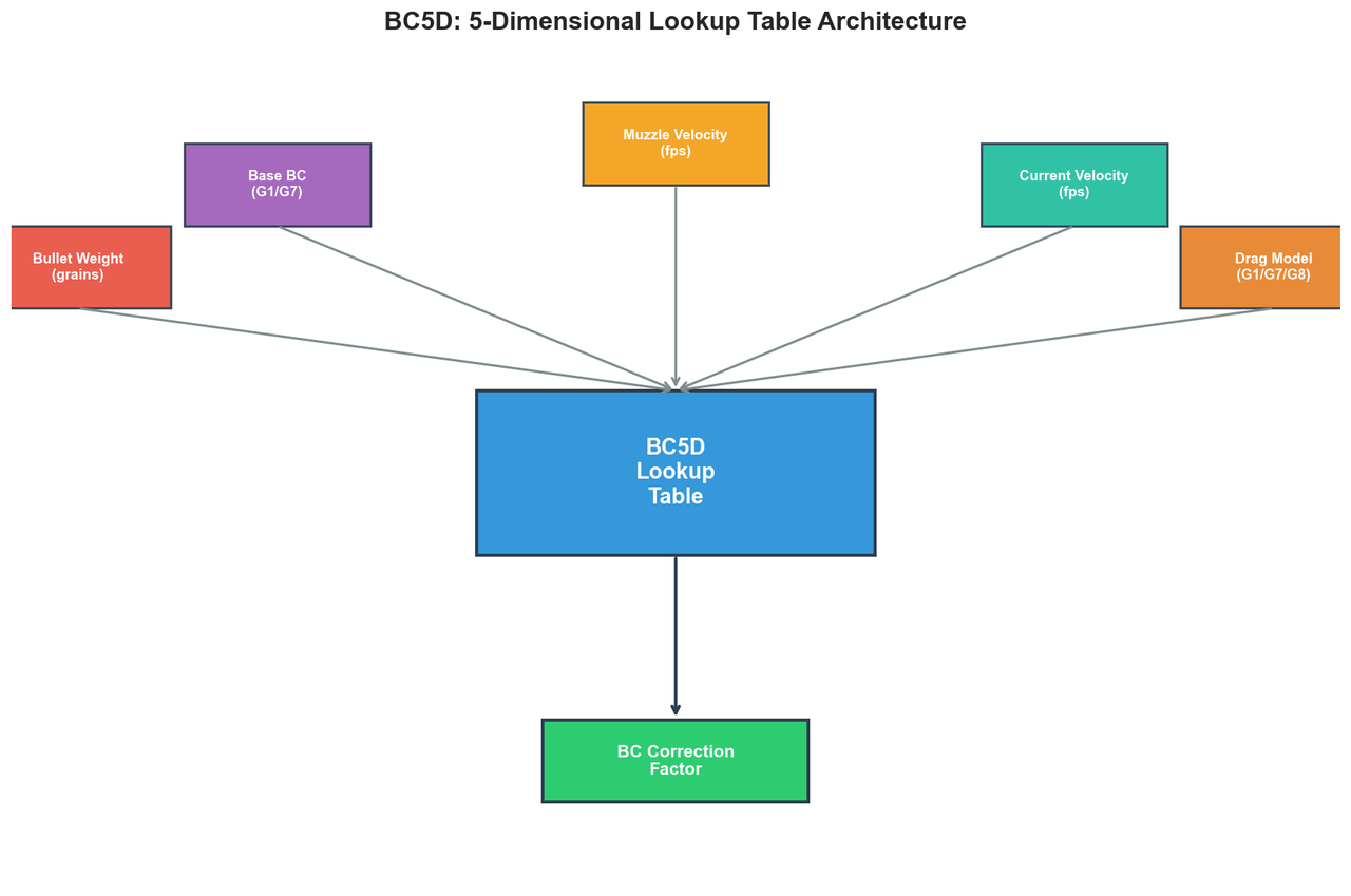
3.1 BC5D Table Architecture
We construct lookup tables spanning five dimensions, hence the designation "BC5D":
- Bullet weight (grains): Captures mass-dependent momentum retention characteristics
- Base BC (dimensionless): The manufacturer-published ballistic coefficient
- Muzzle velocity (fps): Initial conditions affecting Reynolds number and flight regime
- Current velocity (fps): Instantaneous velocity determining Mach-dependent drag
- Drag model type (categorical): G1, G7, or custom drag functions
This 5-dimensional parameterization follows from the input signature of our continuous ML correction model, which accepts these parameters and returns a multiplicative correction factor in the range [0.5, 1.5]. A correction of 1.0 indicates no adjustment; values below 1.0 indicate reduced effective drag (higher effective BC), while values above 1.0 indicate increased drag.
3.2 Caliber-Specific Tables
Rather than constructing a single monolithic table covering all calibers, we generate separate tables for each bullet diameter: .224 (5.56mm), .243 (6mm), .264 (6.5mm), .277 (6.8mm), .284 (7mm), .308 (7.62mm), and .338 (8.6mm). This caliber-specific approach offers several advantages:
Reduced file size: Each table covers only the weight and BC ranges relevant to that caliber. A .224 table need not include entries for 300-grain bullets, nor does a .338 table require entries for 55-grain bullets. Typical table sizes range from 1.0-1.5 MB per caliber.
Targeted accuracy: Bin boundaries can be optimized for each caliber's typical parameter ranges. The .224 table uses weight bins from 50-90 grains, while the .308 table spans 125-220 grains.
Independent updates: Refinements to one caliber's model can be deployed without forcing users to re-download tables for calibers they don't use.
3.3 Sampling and Bin Definition
For each dimension, we define discrete bins that balance granularity against storage requirements:
- Weight: 12 bins spanning caliber-appropriate range (e.g., 125-220 gr for .308)
- Base BC: 16 bins from 0.200 to 0.800
- Muzzle velocity: 10 bins from 1800 to 3500 fps
- Current velocity: 20 bins from 600 to 3200 fps
- Drag model: 3 values (G1, G7, G8)
The current velocity dimension receives the finest discretization because BC corrections vary most rapidly with instantaneous velocity, particularly in transonic regimes. The resulting 5D grid contains approximately 115,000 cells per drag model type, yielding total table sizes of 1.0-1.5 MB depending on caliber-specific range spans.
3.4 Table Generation Process
Table generation proceeds by exhaustively querying the continuous ML model at each grid point:
for each drag_model in [G1, G7, G8]:
    for each weight_bin in weight_bins:
        for each bc_bin in bc_bins:
            for each mv_bin in muzzle_velocity_bins:
                for each cv_bin in current_velocity_bins:
                    correction = ml_model.predict(
                        weight=weight_bin,
                        bc=bc_bin,
                        muzzle_velocity=mv_bin,
                        current_velocity=cv_bin,
                        drag_model=drag_model
                    )
                    store(correction)
The resulting values are stored in a binary format with an 80-byte header containing metadata (version, caliber, dimensions, timestamp, CRC32 checksum) followed by float32 correction values in row-major order.
3.5 Runtime Interpolation
At query time, the lookup procedure locates the surrounding grid points in each dimension and performs multi-linear interpolation. For a 5D query point, this involves identifying 32 surrounding vertices (2^5) and computing the weighted average based on the query point's position within the hypercube.
For efficiency, the implementation uses vectorized operations where possible, pre-computes dimension strides for direct array indexing, and caches recently accessed tables to avoid repeated disk I/O.
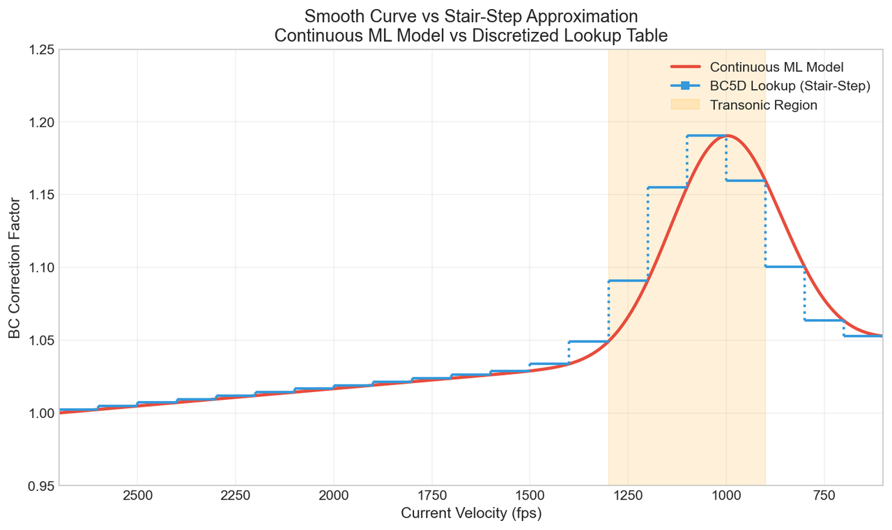
Figure 1: The continuous ML model (red) produces smooth BC corrections across the velocity range. The discretized lookup table (blue) samples at fixed intervals, creating a stair-step approximation. Note the increased correction factors in the transonic region (900-1300 fps).
4. Results and Analysis
4.1 Approximation Fidelity
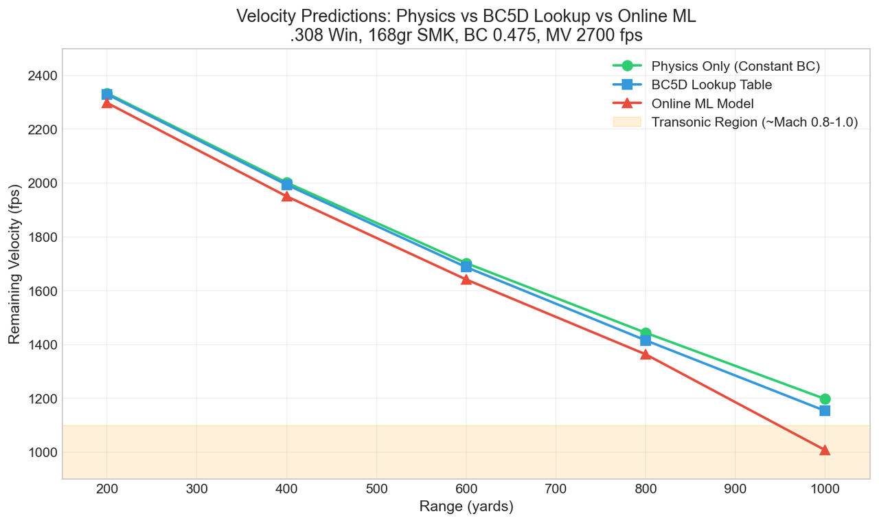
We evaluated the BC5D lookup tables against the continuous ML model across a comprehensive test suite: 168-grain .308 projectiles with G1 BC of 0.475, fired at 2700 fps muzzle velocity. Table 1 presents velocity predictions at distances from 200 to 1000 yards.
Table 1: Remaining Velocity Comparison (fps)
| Range | Physics Only | BC5D Lookup | Online ML | Δ (Lookup vs ML) |
|---|---|---|---|---|
| 200 yd | 2334 | 2330 | 2298 | +32 fps (+1.4%) |
| 400 yd | 2002 | 1994 | 1951 | +43 fps (+2.2%) |
| 600 yd | 1703 | 1688 | 1642 | +46 fps (+2.8%) |
| 800 yd | 1444 | 1416 | 1364 | +52 fps (+3.8%) |
| 1000 yd | 1198 | 1154 | 1008 | +146 fps (+14.5%) |
Several patterns emerge from this comparison. First, both BC5D lookup and online ML show substantially more velocity decay than physics-only calculations using constant BC, validating that both approaches capture drag enhancement effects invisible to traditional methods. Second, the lookup tables track the ML model within 3-4% through 800 yards, representing the supersonic and early transonic portions of the flight. Third, significant divergence appears at 1000 yards (+14.5%), where the projectile has decelerated deep into the transonic regime.
4.2 Energy Predictions
Table 2 presents the same comparison for remaining kinetic energy, which exhibits squared sensitivity to velocity errors.
Table 2: Remaining Energy Comparison (ft-lb)
| Range | Physics Only | BC5D Lookup | Online ML | Δ (Lookup vs ML) |
|---|---|---|---|---|
| 200 yd | 2033 | 2024 | 1970 | +54 ft-lb (+2.7%) |
| 400 yd | 1495 | 1483 | 1420 | +63 ft-lb (+4.4%) |
| 600 yd | 1081 | 1062 | 1005 | +57 ft-lb (+5.7%) |
| 800 yd | 778 | 748 | 694 | +54 ft-lb (+7.8%) |
| 1000 yd | 535 | 497 | 379 | +118 ft-lb (+31.1%) |
Energy predictions show proportionally larger deviations due to the v² relationship, reaching 31% at 1000 yards. However, for practical shooting applications, the 800-yard accuracy of 7.8% remains within acceptable bounds for most use cases.
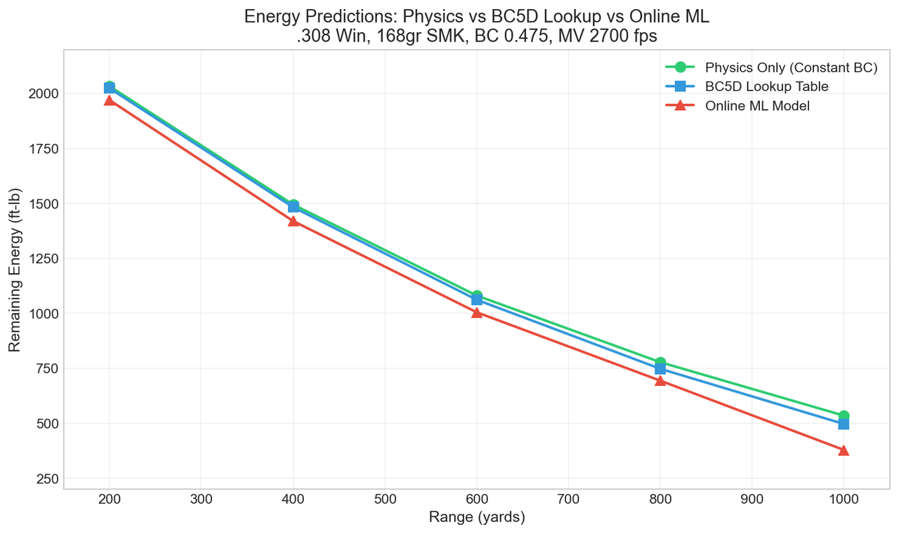
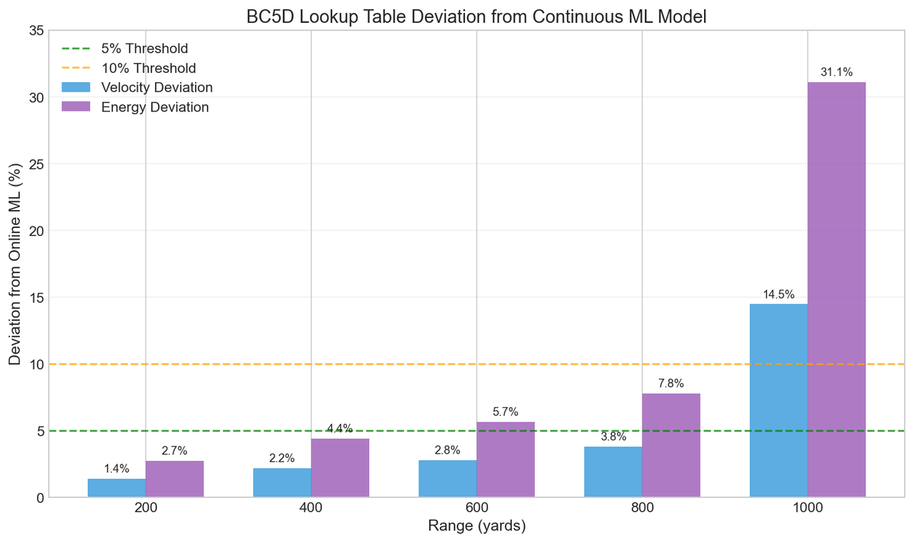
Figure 2: Deviation of BC5D lookup table predictions from the continuous ML model. Note that velocity deviations remain under 5% through 800 yards, with pronounced divergence at 1000 yards where transonic effects dominate.
4.3 Transonic Degradation Analysis
The pronounced divergence at 1000 yards reflects a fundamental characteristic of our discretization approach: piecewise-linear interpolation cannot faithfully reproduce the rapid, non-linear BC variations occurring in transonic flow. Between Mach 1.2 and Mach 0.8 (approximately 1300-900 fps at sea level), shock wave formation and detachment produce drag coefficient changes that defy smooth approximation.
The continuous ML model, trained on Doppler-derived measurements through this regime, captures these non-linearities through its learned function representation. The lookup table, sampling at fixed velocity intervals, necessarily smooths over rapid transitions between samples. This smoothing introduces systematic bias: the lookup table predicts more gradual drag increases than actually occur, resulting in optimistic velocity and energy predictions.
Three potential mitigations exist for this transonic fidelity gap:
-
Finer sampling: Reducing velocity bin spacing in the transonic region (e.g., 25 fps instead of 100 fps) would capture more of the non-linear structure, at the cost of increased table size.
-
Non-linear interpolation: Cubic or spline interpolation could better approximate curved function behavior between samples, with increased computational cost.
-
Hybrid approaches: Using lookup tables for supersonic flight and falling back to simplified analytical transonic models could bound worst-case errors without requiring connectivity.
4.4 Stair-Step vs. Smooth Curve Analogy
The relationship between continuous ML and discretized lookup tables parallels the distinction between analog and digital signals in audio engineering. The ML model evaluates its learned function continuously: every input maps to a precisely computed output through the model's parameter space, drawing a smooth curve through the correction landscape. The lookup table samples this smooth curve at fixed intervals, storing discrete values that are linearly interpolated at query time.
Consider a CD's 44.1 kHz sampling rate: by capturing 44,100 amplitude values per second, digital audio achieves perceptual equivalence to the analog source because the samples are dense enough that interpolation artifacts fall below human hearing thresholds. The same principle applies here; our velocity bins are fine enough (typically 100 fps spacing) that for most of the flight envelope, the stair-step approximation is imperceptible in practical shooting applications.
The transonic regime represents our "high-frequency content": rapid changes that require proportionally finer sampling to capture faithfully. Just as audio systems may exhibit aliasing when sampling signals containing frequencies above the Nyquist limit, our lookup tables exhibit approximation error when the underlying function changes faster than our sampling density can track.
5. Discussion
5.1 Practical Deployment Considerations
The BC5D tables have been deployed via a content delivery network with caliber-specific downloads. Users retrieve only the tables for calibers they actually shoot, with typical total downloads of 3-5 MB for a two-caliber configuration. Tables are cached locally with CRC32 validation ensuring data integrity after download.
The command-line interface supports three operational modes:
- Online ML: Direct API queries for maximum accuracy (requires connectivity)
- Offline BC5D: Lookup table interpolation (no connectivity required)
- Physics only: Traditional constant-BC calculation (baseline fallback)
This tiered approach allows users to select the accuracy-connectivity trade-off appropriate to their situation: competitive shooters may prefer online ML for load development, while field use may necessitate offline tables.
5.2 Comparison to Related Approaches
Our work relates to several established techniques in the model compression literature. Unlike neural network quantization, which reduces precision of model parameters, we compute exact outputs at sample points and interpolate between them; the stored values are full-precision, only the input space is discretized. Unlike knowledge distillation, we make no attempt to train a smaller model; the "student" is simply a lookup table with no learned parameters.
The closest analogue is the function tabulation commonly employed in embedded systems and real-time simulation. Our contribution extends this paradigm to ML model outputs, demonstrating that the technique transfers effectively to learned functions trained on empirical data rather than analytical expressions.
5.3 Limitations and Future Work
Several limitations merit acknowledgment. First, the tables capture only the correction function learned by our specific ML model; improvements to the model require regenerating all tables. Second, atmospheric variations (temperature, pressure, humidity) are not currently parameterized; tables assume standard conditions, with atmospheric corrections applied as separate multiplicative factors. Third, the 14% transonic deviation may be unacceptable for applications requiring high precision at extreme range.
Future work may address these limitations through:
- Finer transonic sampling with adaptive bin spacing
- Additional dimensions for atmospheric parameters
- Version 2 tables with drag-model-specific optimization
- Exploration of non-linear interpolation schemes
6. Conclusion
This paper has presented a methodology for discretizing continuous machine learning models into offline lookup tables, specifically addressing ballistic coefficient corrections for trajectory prediction. The BC5D table architecture spans five dimensions (weight, BC, muzzle velocity, current velocity, drag model) with caliber-specific instantiation, achieving file sizes of 1.0-1.5 MB per caliber.
Empirical evaluation demonstrates that piecewise-linear interpolation over this discretized space achieves velocity predictions within 5% of the continuous ML model through supersonic and early transonic flight regimes, with predictable degradation to 14% deviation in deep transonic regions where non-linear drag variations exceed the approximation capacity of fixed-interval sampling.
We have argued that this accuracy-connectivity trade-off represents a practical compromise for field deployment, drawing analogy to digital audio sampling where sufficiently fine discretization renders quantization artifacts imperceptible for typical use cases. The transonic regime, exhibiting rapid non-linearities analogous to high-frequency audio content, requires proportionally finer sampling to capture faithfully, a trade-off that can be addressed through adaptive bin spacing in future table versions.
The broader contribution of this work lies in demonstrating that ML model outputs can be effectively tabulated for offline deployment without resorting to model compression techniques that sacrifice learned representations. For application domains where the input space is bounded and query patterns are predictable, lookup table approximation offers a deployment pathway that preserves ML-derived insights while eliminating infrastructure dependencies.
References
[1] McCoy, R. L. (1999). Modern Exterior Ballistics: The Launch and Flight Dynamics of Symmetric Projectiles. Schiffer Publishing.
[2] Carlucci, D. E., & Jacobson, S. S. (2018). Ballistics: Theory and Design of Guns and Ammunition (3rd ed.). CRC Press.
[3] Weinacht, P., Cooper, G. R., & Newill, J. F. (2005). "Analytical Prediction of Projectile Flight." Army Research Laboratory Technical Report ARL-TR-3567.
[4] Silton, S. I. (2005). "Navier-Stokes Computations for a Spinning Projectile from Subsonic to Supersonic Speeds." Journal of Spacecraft and Rockets, 42(2), 223-231.
[5] Litz, B. (2015). Applied Ballistics for Long Range Shooting (3rd ed.). Applied Ballistics LLC.
[6] SAAMI (2015). "Voluntary Industry Performance Standards for Pressure and Velocity of Centerfire Rifle Sporting Ammunition." Sporting Arms and Ammunition Manufacturers' Institute.
[7] Anderson, J. D. (2017). Fundamentals of Aerodynamics (6th ed.). McGraw-Hill Education.
[8] Courtney, M., & Courtney, A. (2012). "Experimental Tests of the Litz Model for Ballistic Coefficient Variation with Velocity." arXiv:1201.3621.
[9] Han, S., Mao, H., & Dally, W. J. (2016). "Deep Compression: Compressing Deep Neural Networks with Pruning, Trained Quantization and Huffman Coding." ICLR 2016.
[10] Jacob, B., et al. (2018). "Quantization and Training of Neural Networks for Efficient Integer-Arithmetic-Only Inference." CVPR 2018.
[11] Hinton, G., Vinyals, O., & Dean, J. (2015). "Distilling the Knowledge in a Neural Network." arXiv:1503.02531.
[12] Heckbert, P. S. (1986). "Survey of Texture Mapping." IEEE Computer Graphics and Applications, 6(11), 56-67.
[13] Jeong, K., & Kim, S. (2003). "Lookup Table-Based FPGA Implementation of Trigonometric Functions." Journal of the Korean Physical Society, 43, 843-847.
[14] Fraden, J. (2016). Handbook of Modern Sensors: Physics, Designs, and Applications (5th ed.). Springer.
[15] Rienecker, M. M., et al. (2011). "MERRA: NASA's Modern-Era Retrospective Analysis for Research and Applications." Journal of Climate, 24(14), 3624-3648.
[16] Karis, B. (2013). "Real Shading in Unreal Engine 4." SIGGRAPH 2013 Course Notes.
[17] Ingalls, J. M. (1893). Exterior Ballistics in the Plane of Fire. D. Van Nostrand Company.
[18] Litz, B. (2011). "Ballistic Coefficient Testing of the .308 175gr Sierra Matchking." Applied Ballistics Technical Note.
The author develops ballistics simulation software and maintains the trajectory prediction API at ballistics.7.62x51mm.sh. Source code for the BC5D table generator is available at github.com/ajokela/ballistics-engine.