Discover how the Crank-Nicolson and finite differences methods revolutionized the world of option pricing. In this blog post, we dive deep into these powerful numerical techniques that have become essential tools for quantitative analysts and financial engineers.
We start by exploring the fundamentals of option pricing and the challenges posed by the Black-Scholes-Merton partial differential equation (PDE). Then, we introduce the finite differences method, a numerical approach that discretizes the PDE into a grid of points, enabling us to approximate option prices and calculate crucial risk measures known as the Greeks.
Next, we focus on the Crank-Nicolson method, a more advanced finite difference scheme that combines the best of both explicit and implicit methods. We explain how this method provides second-order accuracy in time and space, ensuring faster convergence and more accurate results.
Through step-by-step explanations and illustrative examples, we demonstrate how these methods are implemented in practice, including the treatment of boundary conditions and the incorporation of the early exercise feature for American options.
Whether you're a curious investor, a financial enthusiast, or an aspiring quantitative analyst, this blog post will provide you with valuable insights into the world of option pricing. Join us as we unravel the secrets behind these powerful numerical methods and discover how they have transformed the way we value and manage options in modern finance.
The Black-Scholes-Merton (BSM) partial differential equation
The Black-Scholes-Merton (BSM) partial differential equation is a mathematical model used for pricing options and other financial derivatives. It was developed by Fischer Black, Myron Scholes, and Robert Merton in the early 1970s and has become a cornerstone of modern financial theory.
Fundamentals of Options Pricing: Options are financial contracts that give the holder the right, but not the obligation, to buy (call option) or sell (put option) an underlying asset at a predetermined price (strike price) on or before a specific date (expiration date). The price of an option depends on several factors, including the current price of the underlying asset, the strike price, the time to expiration, the risk-free interest rate, and the volatility of the underlying asset.
The BSM equation is based on the following assumptions: 1. The market is efficient, and there are no arbitrage opportunities. 2. The underlying asset follows a geometric Brownian motion with constant drift and volatility. 3. The risk-free interest rate is constant and known. 4. There are no transaction costs or taxes. 5. The underlying asset pays no dividends.
Black-Scholes-Merton Partial Differential Equation: The BSM equation describes the price of a European option as a function of time and the underlying asset price. It is a second-order partial differential equation:
Where:
- - V is the option price
- - S is the underlying asset price
- - t is time
- - r is the risk-free interest rate
- - σ is the volatility of the underlying asset
Challenges Posed by the BSM Equation:
-
Volatility Estimation: The BSM equation assumes constant volatility, which is not always the case in real markets. Estimating volatility accurately is crucial for option pricing.
-
Model Assumptions: The assumptions underlying the BSM model, such as no transaction costs and continuous trading, do not hold in practice. This can lead to discrepancies between theoretical and market prices.
-
Numerical Methods: Solving the BSM equation often requires numerical methods, such as finite difference or Monte Carlo simulations, which can be computationally intensive.
-
Market Anomalies: The BSM model does not account for market anomalies, such as the volatility smile or skew, which suggest that implied volatility varies with strike price and time to expiration.
-
Model Extensions: The basic BSM model has been extended to account for dividends, early exercise (for American options), and other factors. These extensions add complexity to the model and its implementation.
Despite these challenges, the Black-Scholes-Merton model remains a foundational tool in options pricing and financial risk management. It provides a framework for understanding the factors that influence option prices and serves as a benchmark for more advanced models.
The Finite Difference Method
The finite difference method is a numerical technique used to solve partial differential equations (PDEs) by approximating derivatives with finite differences. It is particularly useful when analytical solutions are difficult or impossible to obtain. The method discretizes the continuous PDE problem into a discrete set of points in space and time, called a grid or mesh.
To illustrate the basics of the finite difference method, consider a simple one-dimensional heat equation:
Where:
- - u is the temperature
- - t is time
- - x is the spatial coordinate
- - α is the thermal diffusivity
To apply the finite difference method, we discretize the space and time domains into a grid with uniform step sizes Δx and Δt, respectively. We denote the temperature at grid point i and time step n as u(i, n) = u(i Δx, n Δt).
The finite difference method approximates the derivatives using Taylor series expansions. For example, the first-order time derivative can be approximated using the forward difference:
Similarly, the second-order spatial derivative can be approximated using the central difference:
By substituting these approximations into the original PDE, we obtain a system of algebraic equations that can be solved numerically. The finite difference method provides an approximation of the solution at each grid point and time step.
There are various schemes for discretizing time, such as the explicit (forward Euler/01%3A_Chapters/1.02%3A_Forward_Euler_method)), implicit (backward Euler/01%3A_Chapters/1.03%3A_Backward_Euler_method)), and the Crank-Nicolson methods. Each scheme has its own stability, accuracy, and computational requirements.
The finite difference method is widely used in computational finance, particularly in the numerical solution of the Black-Scholes-Merton PDE for option pricing. It is also applied in other fields, such as heat transfer, fluid dynamics, and electromagnetism.
Let's walk through a simple example using the one-dimensional heat equation mentioned earlier. We'll solve the equation numerically using the explicit (forward Euler) finite difference method.
Consider a one-dimensional rod of length L = 1 m, with an initial temperature distribution u(x, 0) = sin(πx) and fixed boundary conditions u(0, t) = u(L, t) = 0. The thermal diffusivity is α = 0.1 m²/s. We'll solve for the temperature distribution over a time period of T = 0.5 s.
Step 1: Discretize the space and time domains Let's divide the rod into N = 10 equally spaced points, with Δx = L / (N - 1) = 0.1 m. We'll use a time step of Δt = 0.01 s, resulting in M = T / Δt = 50 time steps.
Step 2: Set up the initial condition At t = 0, the temperature at each grid point is: u(i, 0) = sin(πx_i), where x_i = i Δx, for i = 0, 1, ..., N-1.
For example:
u(0, 0) = sin(π × 0) = 0
u(1, 0) = sin(π × 0.1) ≈ 0.309
...
u(9, 0) = sin(π × 0.9) ≈ 0.309
u(10, 0) = sin(π × 1) = 0
Step 3: Apply the explicit finite difference scheme For each time step n = 0, 1, ..., M-1 and each interior grid point i = 1, 2, ..., N-2, update the temperature using the explicit scheme:
u(i, n+1) = u(i, n) + α Δt / (Δx)² × [u(i+1, n) - 2u(i, n) + u(i-1, n)]
For example, at the first time step (n = 0) and the first interior grid point (i = 1):
u(1, 1) = u(1, 0) + 0.1 × 0.01 / (0.1)² × [u(2, 0) - 2u(1, 0) + u(0, 0)]
        ≈ 0.309 + 0.1 × [0.588 - 2 × 0.309 + 0] ≈ 0.306
Repeat this process for all interior grid points and time steps, while keeping the boundary conditions fixed at 0.
Step 4: Analyze the results After completing all time steps, you will have approximated the temperature distribution u(x, t) at each grid point and time step. You can visualize the results by plotting the temperature profile at different times or creating an animation showing the evolution of the temperature over time.
Note that the explicit scheme used in this example has a stability condition: α Δt / (Δx)² ≤ 0.5. If this condition is not met, the numerical solution may become unstable and diverge from the actual solution. In such cases, an implicit scheme or a smaller time step may be necessary.
The Crank-Nicolson Method
Let's dive into the Crank-Nicolson method and see how it can be applied to the Black-Scholes-Merton partial differential equation for options pricing.
The Black-Scholes-Merton PDE for a European call option is:
Where:
- - V is the option price
- - S is the underlying asset price
- - t is time
- - r is the risk-free interest rate
- - σ is the volatility of the underlying asset
The Crank-Nicolson method discretizes the PDE using a weighted average of the explicit and implicit schemes, with equal weights of 0.5. This approach results in second-order accuracy in both time and space.
Let's denote the option price at grid point i and time step n as V(i, n) = V(i ΔS, n Δt), where ΔS and Δt are the step sizes in the asset price and time dimensions, respectively.
The Crank-Nicolson scheme for the Black-Scholes-Merton PDE can be written as:
Where:
- - α = 1/2 σ² S_i² Δt / (ΔS)²
- - β = r S_i Δt / (2 ΔS)
- - γ = r Δt / 2
 This scheme leads to a tridiagonal system of linear equations that can be solved efficiently using the Thomas algorithm or other methods for tridiagonal matrices.
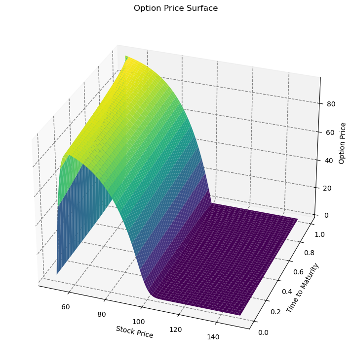
To illustrate the Crank-Nicolson method with an example, consider a European call option with the following parameters:
- - S = 100 (current stock price)
- - K = 100 (strike price)
- - T = 1 (time to maturity in years)
- - r = 0.05 (risk-free interest rate)
- - σ = 0.2 (volatility)
We can discretize the asset price dimension into N = 200 points, with S_min = 0 and S_max = 200, and the time dimension into M = 100 steps.
At each time step, we construct the tridiagonal matrix and solve the resulting system of equations to obtain the option prices at the next time step. The boundary conditions are:
- - V(0, n) = 0 (option value is zero when the stock price is zero)
- - V(N, n) = S_max - K exp(-r(T - n Δt)) (option value at the maximum stock price)
After the final time step, the option price at the initial stock price S is the desired result.
The Crank-Nicolson method provides a stable and accurate solution to the Black-Scholes-Merton PDE. Its second-order accuracy in both time and space ensures faster convergence and more precise results compared to the explicit or implicit methods alone. However, it requires solving a system of equations at each time step, which can be computationally more expensive than the explicit method.
In practice, the Crank-Nicolson method is widely used in financial engineering for options pricing and other applications involving parabolic PDEs. It strikes a balance between accuracy and computational efficiency, making it a popular choice among practitioners.
Crank-Nicolson in Rust as a Python library
Jupyter Notebook for using the python library
extern crate nalgebra as na;
use na::{DMatrix};
use numpy::{PyArray2, PyArray};
use numpy::PyArrayMethods;
use pyo3::prelude::*;
use pyo3::wrap_pyfunction;
use pyo3::exceptions::PyValueError;

/// Constructs a tridiagonal matrix with specified diagonals.
///
/// # Arguments
///
/// * `n` - The size of the matrix.
/// * `a` - The value of the subdiagonal.
/// * `b` - The value of the main diagonal.
/// * `c` - The value of the superdiagonal.
///
/// # Returns
///
/// A tridiagonal matrix with the specified diagonals.
fn tridiag(n: usize, a: f64, b: f64, c: f64) -> DMatrix<f64> {
    let mut mat = DMatrix::<f64>::zeros(n, n);
    for i in 0..n {
        if i > 0 {
            mat[(i, i - 1)] = a;
        }
        mat[(i, i)] = b;
        if i < n - 1 {
            mat[(i, i + 1)] = c;
        }
    }
    mat
}

/// Solves the option pricing problem using the Crank-Nicolson method.
///
/// # Arguments
///
/// * `py` - The Python interpreter instance.
/// * `s0` - Initial stock price.
/// * `k` - Strike price.
/// * `r` - Risk-free rate.
/// * `sigma` - Volatility.
/// * `t` - Time to maturity.
/// * `n` - Number of time steps.
/// * `m` - Number of stock price steps.
///
/// # Returns
///
/// A 2D numpy array containing the option prices.
#[pyfunction]
fn crank_nicolson(
    py: Python,
    s0: f64,
    k: f64,
    r: f64,
    sigma: f64,
    t: f64,
    n: usize,
    m: usize,
) -> PyResult<Py<PyArray2<f64>>> {
    // Time step size
    let dt = t / n as f64;
    // Spatial step size
    let dx = sigma * (t / n as f64).sqrt();
    // Drift term
    let nu = r - 0.5 * sigma.powi(2);
    // Square of spatial step size
    let dx2 = dx * dx;

    // Initialize the grid for option prices
    let mut grid = DMatrix::<f64>::zeros(n + 1, m + 1);

    // Set terminal condition (payoff at maturity)
    for j in 0..=m {
        let stock_price = s0 * (-((m as isize / 2) as f64 - j as f64) * dx).exp();
        grid[(n, j)] = (k - stock_price).max(0.0);
    }

    // Coefficients for the tridiagonal matrices
    let alpha = 0.25 * dt * (sigma.powi(2) / dx2 - nu / dx);
    let beta = -0.5 * dt * (sigma.powi(2) / dx2 + r);
    let gamma = 0.25 * dt * (sigma.powi(2) / dx2 + nu / dx);

    // Construct tridiagonal matrices A and B
    let a = tridiag(m + 1, -alpha, 1.0 - beta, -gamma);
    let b = tridiag(m + 1, alpha, 1.0 + beta, gamma);

    // Perform LU decomposition of matrix A
    let lu = a.lu();

    // Backward time-stepping to solve the PDE
    for i in (0..n).rev() {
        let rhs = &b * grid.row(i + 1).transpose();
        let sol = lu.solve(&rhs).ok_or_else(|| PyValueError::new_err("Failed to solve LU"))?;
        grid.set_row(i, &sol.transpose());
    }

    // Convert DMatrix to Vec<Vec<f64>> for PyArray2
    let rows = grid.nrows();
    let cols = grid.ncols();
    let mut vec_2d = Vec::with_capacity(rows);
    for i in 0..rows {
        let mut row = Vec::with_capacity(cols);
        for j in 0..cols {
            row.push(grid[(i, j)]);
        }
        vec_2d.push(row);
    }

    // Create a numpy array from the Vec<Vec<f64>>
    let array = PyArray::from_vec2_bound(py, &vec_2d).map_err(|_| PyValueError::new_err("Failed to create numpy array"))?;
    Ok(array.unbind())
}

/// Calculates the Greeks (delta, gamma, theta, vega, and rho) for the option.
///
/// # Arguments
///
/// * `py` - The Python interpreter instance.
/// * `s0` - Initial stock price.
/// * `k` - Strike price.
/// * `r` - Risk-free rate.
/// * `sigma` - Volatility.
/// * `t` - Time to maturity.
/// * `n` - Number of time steps.
/// * `m` - Number of stock price steps.
///
/// # Returns
///
/// A tuple containing the values of delta, gamma, theta, vega, and rho.
#[pyfunction]
fn calculate_greeks(
    py: Python,
    s0: f64,
    k: f64,
    r: f64,
    sigma: f64,
    t: f64,
    n: usize,
    m: usize,
) -> PyResult<(f64, f64, f64, f64, f64)> {
    let grid = crank_nicolson(py, s0, k, r, sigma, t, n, m)?;
    let grid = grid.bind(py).readonly();
    let ds = s0 * (sigma * (t / n as f64).sqrt()).exp();
    let dt = t / n as f64;

    let price_idx = m / 2;
    let price = grid.as_slice().unwrap()[price_idx];
    let price_up = grid.as_slice().unwrap()[price_idx + 1];
    let price_down = grid.as_slice().unwrap()[price_idx - 1];

    // Calculate delta, gamma, and theta
    let delta = (price_up - price_down) / (2.0 * ds);
    let gamma = (price_up - 2.0 * price + price_down) / (ds * ds);
    let theta = (grid.as_slice().unwrap()[price_idx + 1] - price) / dt;

    // Calculate vega
    let eps = 0.01;
    let sigma_vega = sigma + eps;
    let grid_vega = crank_nicolson(py, s0, k, r, sigma_vega, t, n, m)?;
    let grid_vega = grid_vega.bind(py).readonly();
    let price_vega = grid_vega.as_slice().unwrap()[price_idx];
    let vega = (price_vega - price) / eps;

    // Calculate rho
    let r_rho = r + eps;
    let grid_rho = crank_nicolson(py, s0, k, r_rho, sigma, t, n, m)?;
    let grid_rho = grid_rho.bind(py).readonly();
    let price_rho = grid_rho.as_slice().unwrap()[price_idx];
    let rho = (price_rho - price) / eps;

    Ok((delta, gamma, theta, vega, rho))
}

/// Extracts the option price from the grid at the initial time step for the given parameters.
///
/// # Arguments
///
/// * `py` - The Python interpreter instance.
/// * `grid` - The option price grid.
/// * `_s0` - Initial stock price (not used).
/// * `_k` - Strike price (not used).
/// * `_r` - Risk-free rate (not used).
/// * `_sigma` - Volatility (not used).
/// * `_t` - Time to maturity (not used).
/// * `_n` - Number of time steps (not used).
/// * `m` - Number of stock price steps.
///
/// # Returns
///
/// The option price at the initial time step.
#[pyfunction]
fn extract_option_price(
    py: Python,
    grid: Py<PyArray2<f64>>,
    m: usize,
) -> PyResult<f64> {
    let grid = grid.bind(py).readonly();
    // Assuming s0 is near the middle of the grid
    let price_idx = m / 2;
    Ok(grid.as_slice().unwrap()[price_idx])
}

/// Module definition for the finite_differences_options_rs Python module.
#[pymodule]
fn libfinite_differences_options_rs(_py: Python, m: &PyModule) -> PyResult<()> {
    m.add_function(wrap_pyfunction!(crank_nicolson, m)?)?;
    m.add_function(wrap_pyfunction!(calculate_greeks, m)?)?;
    m.add_function(wrap_pyfunction!(extract_option_price, m)?)?;
    Ok(())
}