The Revolutionary Motorola 68000 Microprocessor
 In the annals of computing history, few microprocessors stand out as prominently as the Motorola 68000. This silicon marvel, often referred to simply as the "68k," laid the foundation for an entire generation of computing, playing a seminal role in the development of iconic devices ranging from the Apple Macintosh to the Commodore Amiga, and from the Sega Genesis to the powerful workstations of the 1980s, like the Sun-1 workstation, introduced by Sun Microsystems in 1982.
Inception and Background
Introduced to the world in 1979 by Motorola Semiconductor Products Sector, the Motorola 68000, a family of 32-bit complex instruction set computer (CISC) microprocessors, emerged as a direct response to the demand for more powerful and flexible CPUs. For a trip back in time, checkout this The Computer Chronicles from 1986 on RISC vs. CISC architectures video. The 1970s witnessed an explosion of microprocessor development, with chips like the Intel 8080 - introduced in 1974, the MOS Technology 6502 - introduced in 1975, and the Zilog Z80 - introduced in 1976, shaping the first wave of personal computers. But as the decade drew to a close, there was a noticeable need for something more: a processor that could handle the increasing complexities of software and pave the way for the graphical user interface and multimedia era The m68k was one of the first widely available processors with a 32-bit instruction set, large unsegmented address space, and relatively high speed for the era. As a result, it became a popular design through the 1980s, and was used in a wide variety of personal computers, workstations, and embedded systems.
The m68k has a rich instruction set that includes a variety of features for both general-purpose and specialized applications. For example, the m68k has instructions for floating-point arithmetic, bit manipulation, and memory management. It also has a number of instructions for handling interrupts and exceptions.
The m68k is a well-documented and well-supported processor. There are a number of compilers and development tools available for the m68k, and it is supported by a variety of operating systems, including Unix, Linux, and macOS.
The m68k is still in use today, albeit to a lesser extent than it was in the 1980s and 1990s. It is still used in some embedded systems, and it is also used in some retrocomputing projects.
The 68k's Distinction
Several factors distinguished the 68k from its contemporaries. At the heart of its design was a 32-bit internal architecture. This was a significant leap forward, as many microprocessors of the era, including its direct competitors, primarily operated with 8-bit or 16-bit architectures. This expansive internal data width allowed the 68k to manage larger chunks of data at once and perform computations more efficiently.
Yet, in a nod to compatibility and cost-effectiveness, the 68k featured a 16-bit external data bus and a 24-bit address bus. This nuanced approach meant that while the chip was designed with a forward-looking architecture, it also remained accessible and affordable for its intended market.
Here's a deeper look into the distinct attributes that set the 68k apart:
-
32-bit Internal Architecture: At its core, the 68k was designed as a 32-bit microprocessor, which was a visionary move for its time. While many competing processors like the Intel 8086 and Zilog Z8000 were primarily 16-bit, the 68k's 32-bit internal data paths meant it could process data in larger chunks, enabling faster and more efficient computation. This internal width was a signal to the industry about where the future of computing was headed, and the 68k was at the forefront.
-
Hybrid Bus System: Despite its 32-bit internal prowess, the 68k was pragmatic in its external interfacing. It featured a 16-bit external data bus and a 24-bit address bus. This choice was strategic: it allowed the 68k to communicate with the then-available 16-bit peripheral devices and memory systems, ensuring compatibility and reducing system costs. The 24-bit address bus meant it could address up to 16 megabytes of memory, a generous amount for the era.
-
Comprehensive Instruction Set: One of the crowning achievements of the 68k was its rich and versatile instruction set. Starting with 56 instructions, it was not just about the number but the nature of these instructions. They were designed to be orthogonal, meaning instructions could generally work with any data type and any addressing mode, leading to more straightforward assembly programming and efficient use of the available instruction set. This design consideration provided a more friendly and versatile environment for software developers.
-
Multiple Register Design: The 68k architecture sported 16 general-purpose registers, split equally between data and address registers. This was a departure from many contemporaneous designs that offered fewer registers. Having more registers available meant that many operations could be performed directly in the registers without frequent memory accesses, speeding up computation significantly.
-
Forward-Thinking Design Philosophy: Motorola designed the 68k not just as a response to the current market needs but with an anticipation of future requirements. Its architecture was meticulously crafted to cater to emerging multitasking operating systems, graphical user interfaces, and more complex application software. This forward-leaning philosophy ensured that the 68k remained relevant and influential for years after its debut.
-
Developer and System Designer Appeal: The 68k's design was not just about raw power but also about usability and adaptability. Its clean, consistent instruction set and powerful addressing modes made it a favorite among software developers. For system designers, its compatibility with existing 16-bit components and its well-documented interfacing requirements made it a practical choice for a wide range of applications.
Redefining an Era
But perhaps what truly set the 68k apart from its peers was not just its technical specifications but its broader philosophy. Where many processors of the era were designed with a focus on backward compatibility, the 68k looked forward. It was built not just for the needs of the moment, but with an eye on the future: a future of graphical user interfaces, multimedia applications, and multitasking environments. In the context of the late 1970s and early 1980s, the Motorola 68000 was a beacon of innovation. Its architecture represented a departure from many conventions of the time, heralding a new wave of computing possibilities.
In the vibrant landscape defined by the Motorola 68000's influential reign, there exists a contemporary 68k tiny computer: the Tiny68K, a modern homage to this iconic microprocessor. A compact, single-board computer embodies the 68k's forward-thinking design philosophy, serving both as an educational tool and a nostalgic nod to the golden age of computing. Equipped with onboard RAM, ROM, and serial communication faculties, the Tiny68K is more than just a tribute; it's a hands-on gateway for enthusiasts and students to dive deep into the 68k architecture. By offering a tangible platform for assembly programming and hardware design exploration, the Tiny68K seamlessly marries the pioneering spirit of the 68k era with the curiosity of contemporary tech enthusiasts.
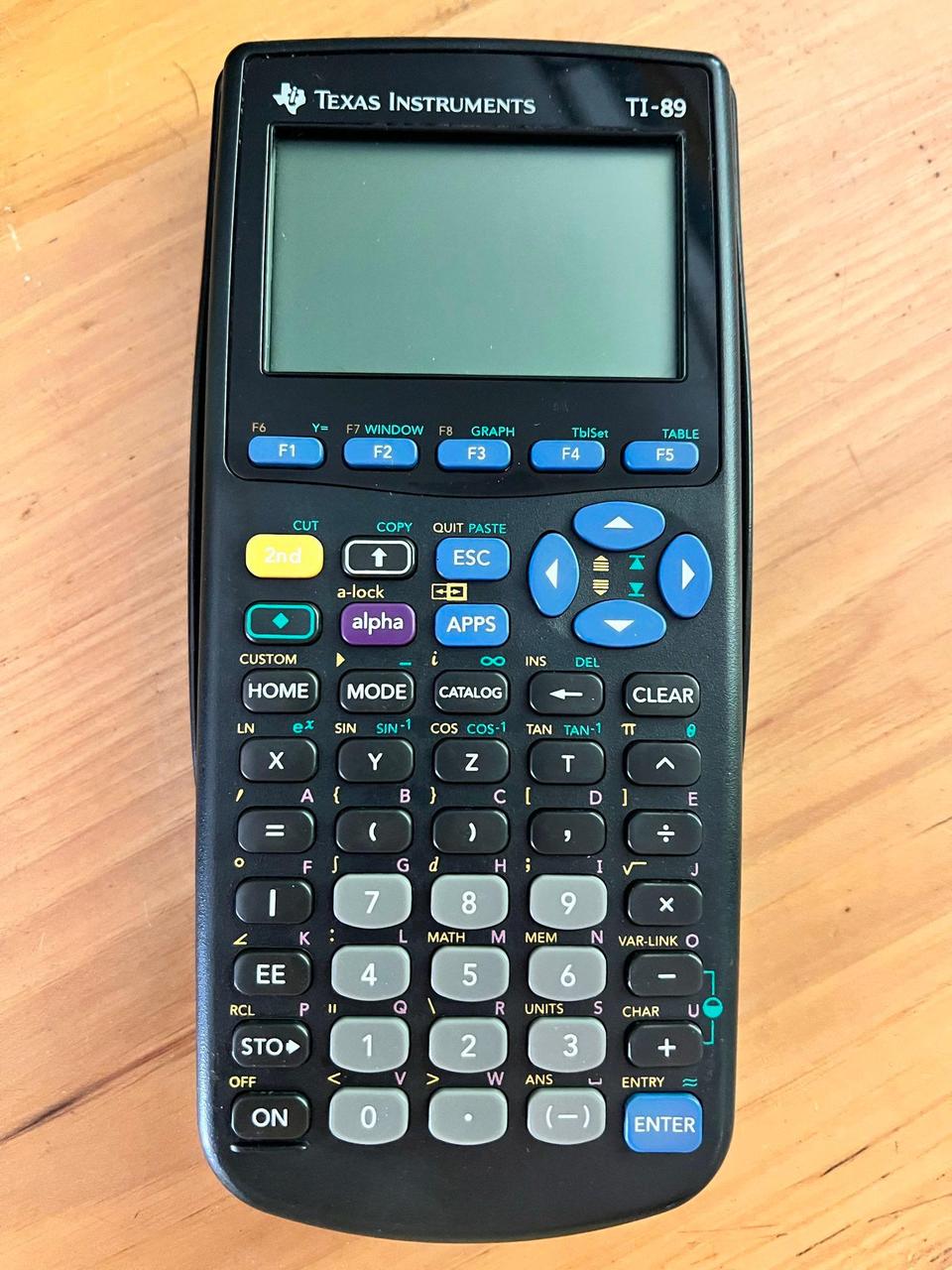
But, if we step back two and a half decades from the contemporary Tiny68k, you will find the Texas Instruments TI-89 graphing calculator. Launched in the late 1990s, and predating the TI-84+ by several years, the TI-89 represented a significant leap forward in handheld computational capability for students and professionals. While the 68k had already etched its mark in workstations and desktop computers, its adoption into the TI-89 showcased its versatility and longevity. This wasn't just any calculator; it was a device capable of symbolic computation, differential equations, and even 3D graphing, functionalities akin to sophisticated computer algebra systems, but fitting snugly in one's pocket. The choice of the 68k for the TI-89 wasn't merely a hardware decision; it was a statement of intent, bringing near-desktop-level computational power to the classroom. The TI-89, with its 68k heart, became an indispensable tool for millions of students worldwide. In this manner, the 68k's legacy took a pedagogical turn, fostering learning and scientific exploration in academic settings globally, further cementing its storied and diverse contribution to the world of computing.
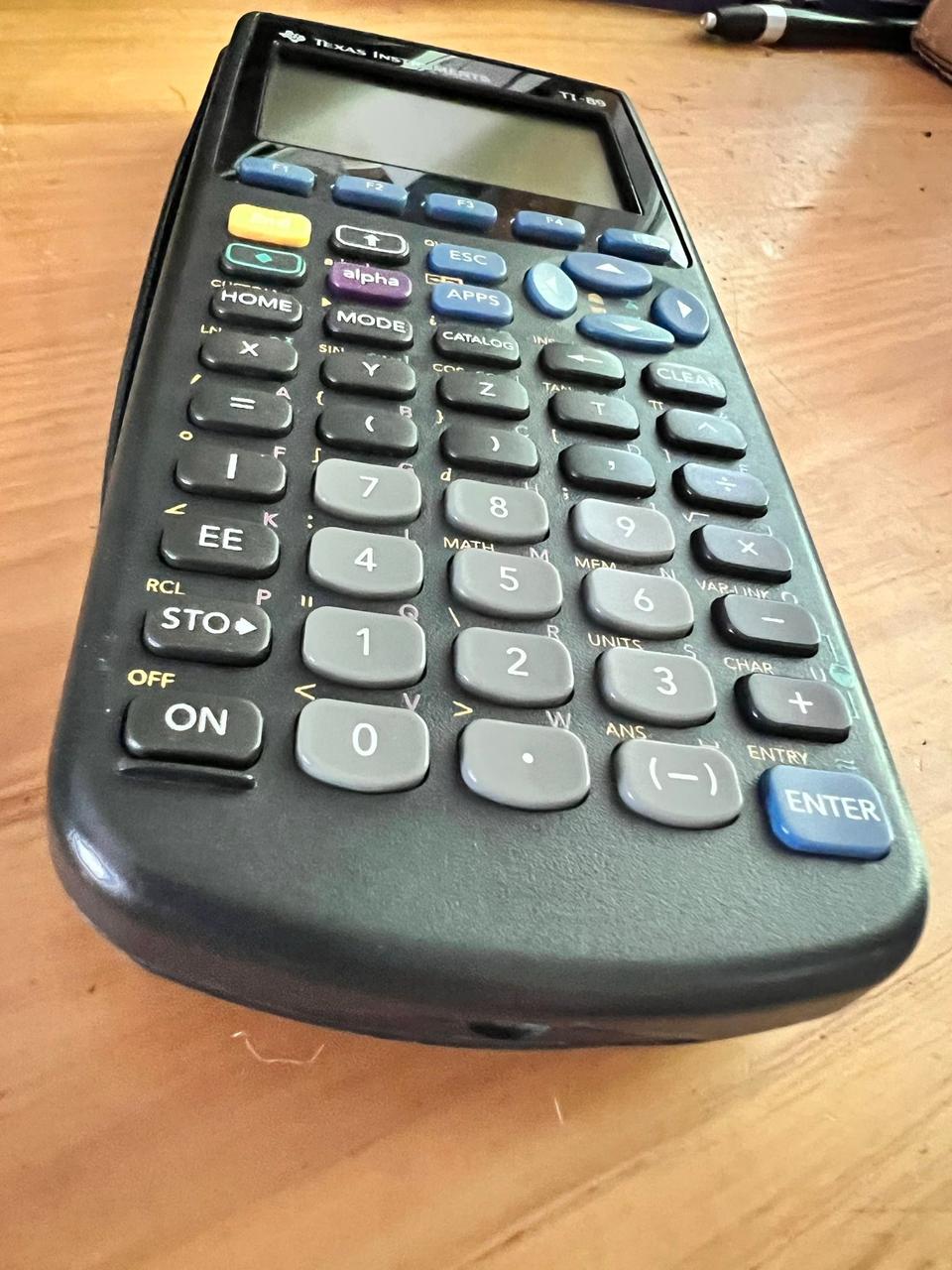 During the late 1990s and early 2000s, as I delved into the foundational calculus studies essential for every engineering and computer science student, I invested in a TI-89. Acquiring it with the savings from my college job, this graphing calculator, driven by the robust 68k architecture, swiftly became an invaluable tool. Throughout my undergraduate academic journey, the TI-89 stood out not just as a calculator, but as a trusted companion in my studies. From introductory calculus to multivariate calculus to linear algebra and differential equations, my TI-89 was rarely out of reach while in the classroom.
The TI-89 was not the only device in my backpack. At the same time in my schooling, my undergraduate university, the University of Minnesota Duluth (UMD), took, what was at the time, a pioneering step in using technology integrated into the education process. In 2001, the university instituted the forward-thinking requirement for its science and engineering students: the ownership and use of an HP iPAQ. Laptops, at the time, were not seen as being universal like they are now. The College of Science and Engineering felt the iPAQ would be a good choice.
In 2001, the popular models of the HP iPAQ were the H3600 series. These iPAQs were powered by the Intel StrongARM SA-1110 processor, which typically ran at 206 MHz. The StrongARM was a low-power, high-performance microprocessor that made it particularly suitable for mobile devices like the iPAQ, providing a balance between performance and battery life.
The StrongARM microprocessor was a result of collaboration between ARM Ltd. and Digital Equipment Corporation (DEC) in the mid-1990s. It was developed to combine ARM's architectural designs with DEC's expertise in high-performance processor designs.
The processor was based on the ARM v4 architecture, a derivative of the RISC design. It operated at speeds between 160 MHz to 233 MHz and was notable for its minimal power consumption, making it ideal for mobile and embedded systems. Some models consumed as little as 1 mW/MHz. With a performance rate nearing 1 MIPS per MHz, it was designed for high-performance tasks. Manufactured using a 0.35-micron CMOS process, the StrongARM featured a 32-bit data and address bus, incorporated both instruction and data cache, and came with integrated features like memory management units. It was widely used in devices like the iPAQ, various embedded systems, and network devices. Though its production lifespan was relatively short after DEC's acquisition by Intel, the StrongARM significantly showcased the capabilities of ARM designs in merging high performance with power efficiency.
By most measurements, the HP iPAQ and its StrongARM processor had more processing power, more memory, and a subjectively more modern user interface; despite these impressive characteristics, the requirement and use of the device at UMD was short lived. Among a number of issues, connectivity and available software were problems that made the iPAQ program fall short. Often, it couldn't be used on tests, it did not readily have software for symbolic algebra and calculus, and despite having a subjectively snappier UI, devices like the TI-89 (and others in the TI-8x family) had far more intuitive user interface navigation without the need for a stylus pen. By the fall of 2002, I was no longer carrying around this extra device.
The TI-89 was simply better suited for the engineer-in-training. The TI-89 bridged the gap between abstract theoretical concepts and tangible results. But there was more to the device. The TI-89's programmable nature ushered in a culture of innovation. Students and enthusiasts alike began developing custom applications, ranging from utilities to assist in specific academic fields to games that offered a brief respite from rigorous studies. This inadvertently became an entry point for many into the world of programming and software development.
The legacy of the TI-89 extends beyond its lifespan. It's seen in the modern successors of graphing calculators and educational tools that continue to be inspired by its pioneering spirit. It's remembered fondly by a generation who witnessed firsthand the transformative power of integrating cutting-edge technology into education.
Here are some highlights of the TI-89:
-
Memory Architecture: The TI-89 was no slouch when it came to memory, boasting around 256 KB of Flash ROM and 188 KB of RAM in its initial versions. This generous allocation, especially for a handheld device of its era, allowed for advanced applications, expansive user programs, and data storage.
-
RAM (Random Access Memory): The TI-89 features 256 KB (kilobytes) of RAM. This type of memory is used for active calculations, creating variables, and running programs. It can be cleared or reset, which means data stored in RAM is volatile and can be lost if the calculator is turned off or resets.
-
Flash ROM (Read-Only Memory): The TI-89 boasts 2 MB (megabytes) of Flash ROM. This memory is non-volatile, meaning that data stored here remains intact even if the calculator is turned off. Flash ROM is primarily used to store the calculator's operating system, apps, and other user-installed content. Because it's "flashable," the OS can be updated, and additional apps can be added without replacing any hardware.
-
Archive Space: A portion of the Flash ROM (usually the majority of it) is used as "archive" space. This is where users can store programs, variables, and other data that they don't want to lose when the calculator is turned off or if the RAM is cleared.
-
-
Display Capabilities: A 160x100 pixel LCD screen was central to the TI-89's interface. This high-resolution display was capable of rendering graphs, tables, equations, and even simple grayscale images. It was instrumental in visualizing mathematical concepts, from 3D graphing to differential equation solutions.
-
Input/Output (I/O) Interfaces: The TI-89 was equipped with an I/O port, enabling connection with other calculators, computers, or peripheral devices. This feature facilitated data transfer, software upgrades, and even collaborative work. Additionally, the calculator could be connected to specific devices like overhead projectors for classroom instruction, further emphasizing its role as an educational tool.
-
Operating System and Software: The calculator ran on an advanced operating system that supported not only arithmetic and graphing functionalities but also symbolic algebra and calculus. Furthermore, the TI-89 could be programmed in its native TI-BASIC language or with m68k assembly, offering flexibility for developers and hobbyists alike. We will go into the OS in more detail later in this write-up.
-
Expandability: One of the distinguishing features of the TI-89 was its ability to expand its capabilities through software. Texas Instruments, along with third-party developers, created numerous applications for a range of academic subjects, from physics to engineering to finance. Its programmable nature also allowed students and enthusiasts to write custom programs tailored to their needs.
-
Hardware Extensions: Over the years, peripheral hardware was developed to extend the capabilities of the TI-89. This included items like memory expansion modules, wired and wireless communication modules, and even sensors for data collection in scientific experiments.
-
Power Management: The TI-89 was designed for efficient power management. Relying on traditional AAA batteries and a backup coin cell battery to retain memory during main battery replacement, it optimized power usage to ensure long operational periods, essential for students during extended classes or examination settings.
The Business Side
The graphing calculator market possesses several unique characteristics. At its core, the market is oligopolistic in nature, with just a handful of brands like Texas Instruments, Casio, and Hewlett-Packard taking center stage. This structure not only restricts consumer choices but also provides these companies with considerable clout over pricing and product evolution.
A significant factor for these devices is the stable demand they enjoy, primarily driven by their use in high school and college mathematics courses. Year after year, there's a consistent need for these tools, ensuring a predictable market. In terms of technological evolution, the graphing calculator hasn't witnessed revolutionary changes. However, there are discernible improvements, such as the integration of color screens, rechargeable batteries, and augmented processing capabilities in newer models. Another dimension to the equation is the regulatory environment, especially in the context of standardized testing. Only particular calculators are permitted in such settings, which can heavily impact the popularity of specific models among students. Yet, as technology advances, these traditional devices face stiff competition from modern smartphone apps and software offering similar functionalities. Although regulations and educational preferences keep dedicated devices relevant, the growing digital ecosystem poses a formidable challenge.
Pricing in this market is interesting as well. Given their essential role in education, these calculators exhibit a degree of price inelasticity. Students, when presented with a need for a specific model by their institutions, often have little choice but to purchase it, irrespective of minor price hikes. This brings us to another vital market feature: the influence of educational institution recommendations. Schools and colleges often have a say in the models or brands their students should buy, like my undergraduate requirement to have an HP iPAQ, thereby significantly shaping purchase decisions.
Prior to 2008, Texas Instruments broke out their Education Technologies business into its own line item in Securities & Exchange Commission (SEC) 10-Q filings. Education Technologies was primarily concerned with graphing calculators. In 2009, the Wall Street Journal highlighted that Texas Instruments dominated the US graphing calculator market, accounting for roughly 80% of sales. Meanwhile, its rival, Hewlett-Packard (HP), secured less than 5% of this market share. The report further revealed that for all of 2007, calculator sales contributed $526 million in revenues and $208 million in profits to TI, making up about 5% of the company's yearly profits. TI has since rolled their Education Technologies division into an "Other" category on their SEC filings. Even without explicitly calling out its graphing calculators business, their technology remains a mainstay in the educational-industrial complex that is the secondary education system in the US. For a student opinion on the monopolistic grip TI has on the market, check out this.
Texas Instruments Operating System
The TI-89, one of Texas Instruments' advanced graphing calculators, operates on the TI-OS (Texas Instruments Operating System), which offers a slew of sophisticated features catering to high-level mathematics and science needs. The TI-OS provides symbolic manipulation capabilities, allowing users to solve algebraic equations, differentiate and integrate functions, and manipulate expressions in symbolic form. It supports multiple graphing modes, including 3D graphing and parametric, polar, and sequence graphing. The system comes equipped with a versatile programming environment, enabling users to write their custom programs in TI-BASIC or Assembly (as was previously mentioned above). Additionally, the OS incorporates advanced calculus functionalities, matrix operations, and differential equations solvers. It also boasts a user-friendly interface with drop-down menus, making navigation intuitive and efficient.
Beyond the aforementioned features, the TI-89's TI-OS also extends its capabilities to advanced mathematical functions like Laplace and Fourier transforms, facilitating intricate engineering and physics calculations. The calculator’s list and spreadsheet capabilities permit data organization, statistical calculations, and regression analysis. Its built-in Computer Algebra System (CAS) is particularly noteworthy, as it can manipulate mathematical expressions and equations, breaking them down step by step – a godsend for students trying to understand complex mathematical procedures.
In terms of usability, the OS supports a split-screen interface, enabling simultaneous graph and table viewing. This becomes especially helpful when analyzing functions and their respective data points side by side. The operating system also supports the ability to install and utilize third-party applications, expanding the calculator's functionality according to the user's requirements.
Connectivity-wise, TI-OS facilitates data transfers between calculators and to computers. This makes it easier for students and professionals to share programs, functions, or data sets. Moreover, with the integration of interactive geometry software, users can explore mathematical shapes and constructions graphically, fostering a more interactive learning environment. Overall, the TI-89's TI-OS is a robust system that merges comprehensive mathematical tools with user-centric design, making complex computations and data analysis both effective and intuitive.
Writing Software on the TI-89
Let's outline a simple Monte Carlo method to estimate π:
The basic idea of the Monte Carlo method is to randomly generate points inside a square and determine how many fall inside a quarter-circle inscribed within that square. The ratio of points that fall inside the quarter-circle to the total number of points generated will approximate π/4. Isn't math just magical?
Here's a rudimentary outline:
- Create a square with sides of length 2 (so it ranges from -1 to 1 on both axes).
- The quarter-circle within the square is defined by the equation: $$( x^2 + y^2 ≤ 1 )$$
- Randomly generate points (x, y) within the square.
- Count how many points fall within the quarter-circle.
If you generate N points and M of them fall inside the quarter-circle, then the approximation for π is:
$$[ \pi ≈ 4 \times \frac{M}{N} ]$$
Here's a basic implementation in TI-BASIC:
: Prompt N   ; Ask the user for the number of iterations.
: 0→M        ; Initialize M, the number of points inside the quarter-circle.
: For(I,1,N) ; Start a loop from 1 to N.
: rand→X     ; Generate a random number for the x-coordinate between 0 and 1.
: rand→Y     ; Generate a random number for the y-coordinate between 0 and 1.
: If X^2 + Y^2 ≤ 1  ; Check if the point (X, Y) lies inside the quarter-circle.
: M + 1→M    ; If it does, increment the count M.
: End        ; End the loop.
: 4*M/N→P    ; Calculate the approximation for π.
: Disp "Approximation for π:", P  ; Display the result.
When you run this program, you'll input the number of random points (N) to generate. More points will give a more accurate approximation, but the program will run longer. The rand function in TI-BASIC returns a random number between 0 and 1, which is ideal for this method.
Here's a basic M68k assembly outline for the TI-89 (please note this is a high-level, pseudo-code-style representation, as creating an exact and fully functional assembly code requires a more detailed approach):
This was written with the generous help of ChatGPT
    ORG     $0000                   ; Starting address (set as needed)

MonteCarloPi:
    ; Initialize your counters and total points (iterations)
    MOVE.L  #TOTAL_POINTS, D2       ; D2 will be our total iteration counter
    CLR.L   D3                      ; D3 will be our "inside circle" counter

Loop:
    ; Generate random x and y in the range [-1,1]
    JSR     GenerateRandom
    FMOVE   FP0, FP2                ; FP2 is our x-coordinate
    JSR     GenerateRandom
                                  ; FP0 is our y-coordinate

    ; Compute distance from (0,0): sqrt(x^2 + y^2)
    FMUL    FP2, FP2                ; x^2
    FMUL    FP0, FP0                ; y^2
    FADD    FP0, FP2                ; x^2 + y^2
    FSQRT   FP2, FP0                ; sqrt(x^2 + y^2)

    ; Check if point lies inside the circle of radius 1
    FCMP    #1, FP0
    FBLT    InsideCircle            ; If distance < 1, it is inside the circle

    ; Update counters
    SUBQ.L  #1, D2
    BNE     Loop
    BRA     ComputePi

InsideCircle:
    ADDQ.L  #1, D3                  ; Increment the inside circle counter
    BRA     Loop

ComputePi:
    ; Calculate pi: 4 * (points inside circle / total points)
    ; Assuming D3 and D2 are long, this operation will be integer-based, which will result in 0 or 1.
    ; We can multiply D3 by 4 beforehand to get an integer estimate of pi.

    ASL.L   #2, D3                  ; D3 = D3 * 4
    DIVS    D2, D3                  ; Divide by total points (D2)

    ; Convert the result to a string
    MOVE.L  D3, D0
    JSR     IntToStr                ; Result string will be in A1

    ; Display the result (or do whatever you wish with A1)
    ; ...

    RTS


; RNG using Linear Congruential Generator
GenerateRandom:
    MOVE.L  SEED, D0            ; Load current seed into D0
    MULU.L  #A, D0              ; Multiply seed by 'a'
    ADD.L   #C, D0              ; Add 'c'
    DIVU    #M, D0              ; Divide by M. Remainder in D1
    MOVE.L  D1, SEED            ; Store new seed
    MOVE.L  D1, D0              ; Return value in D0
    RTS

IntToStr:
    ; Input: D0 = Integer value to be converted
    ; Output: A1 = Pointer to the resulting string

    LEA     buffer(PC), A0          ; A0 points to end of buffer (for null-terminated string)
    MOVE.B  #0, (A0)                ; Null-terminate

    TST.L   D0                      ; Test if D0 is zero
    BNE     NotZero                 ; If not, proceed with conversion
    MOVE.B  #'0', -1(A0)           ; Store '0' character
    MOVEA.L A0, A1                  ; Move pointer to result
    SUBA.L  #1, A1                  ; Adjust to point at the '0' character
    RTS

NotZero:
    ; Handle negative numbers
    TST.L   D0
    BPL     Positive
    NEG.L   D0
    MOVE.B  #'-', -1(A0)
    SUBA.L  #1, A0

Positive:
    ; Convert each digit to a character

LoopConvert:
    DIVU    #10, D0                 ; Divide by 10, quotient in D0, remainder in D1
    ADD.B   #'0', D1                ; Convert to ASCII
    MOVE.B  D1, -1(A0)              ; Store character at next position in buffer
    SUBA.L  #1, A0                  ; Move buffer pointer backwards
    TST.L   D0                      ; Check if quotient is zero
    BNE     LoopConvert             ; If not, continue loop

    MOVEA.L A0, A1                  ; Move pointer to result string to A1
    RTS

buffer  DS.B    12                  ; Allocate space for max 32-bit number + null-terminator

TOTAL_POINTS  EQU  100000           ; Number of iterations for Monte Carlo (change as needed)
An actual implementation may require adjusting the code, especially if wanting to make use of system routines to display your shiny new approximation of π. Unless you are trying to squeeze out more performance, writing in m68k assembly is not really practical. You are having to track everything manually. Higher level languages were designed to not have to deal with such low level commands. Let's look at C using an older port of the ubiquitous GNU GCC. Don't hold yourself for a porting of Rust to TI-89.
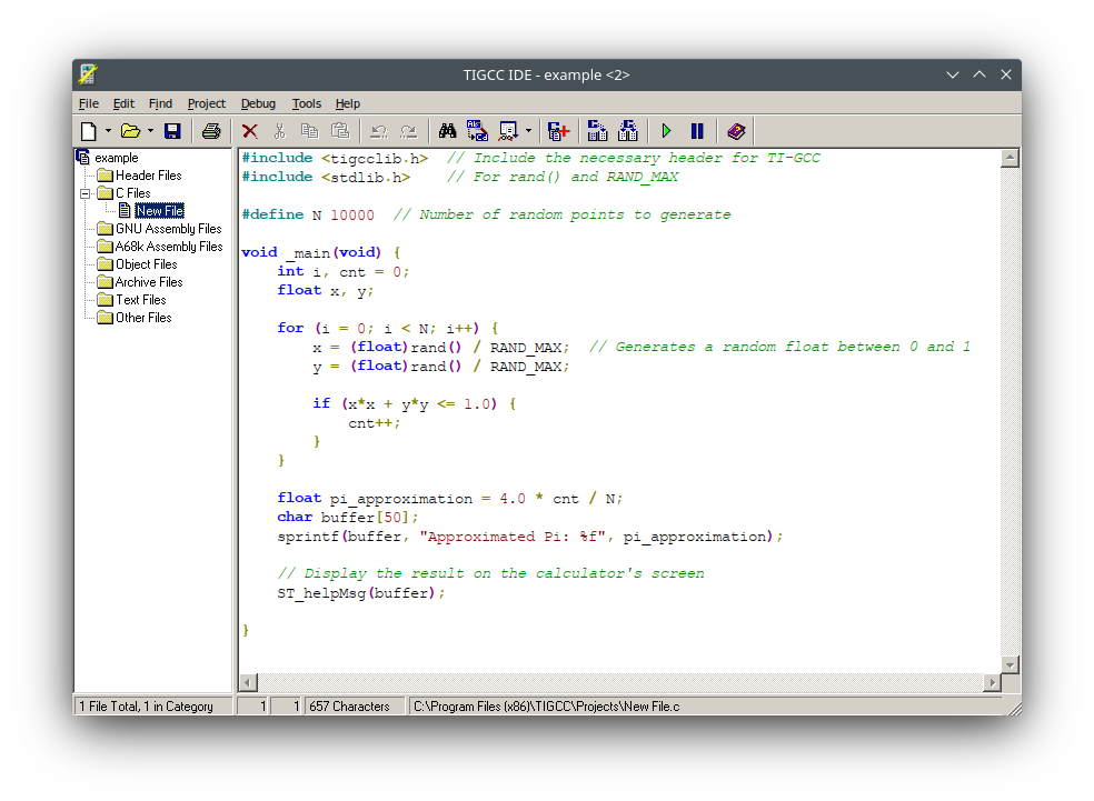
Use the TI-GCC SDK for the TI-89 to write a C program, the Monte Carlo method for estimating the value of π would look like the following block of code. TI-GCC is Windows only, but will install and run quite well under Linux + Wine; I was even able to get these Win32 executables to run on Apple M2 Silicon hardware using wine-crossover.
#include <tigcclib.h>  // Include the necessary header for TI-GCC
#include <stdlib.h>    // For rand() and RAND_MAX

#define N 10000  // Number of random points to generate

void _main(void) {
    int i, cnt = 0;
    float x, y;

    for (i = 0; i < N; i++) {
        x = (float)rand() / RAND_MAX;  // Generates a random float between 0 and 1
        y = (float)rand() / RAND_MAX;

        if (x*x + y*y <= 1.0) {
            cnt++;
        }
    }

    float pi_approximation = 4.0 * cnt / N;
    char buffer[50];
    sprintf(buffer, "Approximated Pi: %f", pi_approximation);

    // Display the result on the calculator's screen
    ST_helpMsg(buffer);

}
This program does the following:
The code begins by including necessary headers and defining a macro, N, to denote the number of random points (10,000) that will be generated. Within the main function _main, two random floating-point numbers between 0 and 1 are generated for each iteration, representing the x and y coordinates of a point. The point's distance from the origin is then checked to determine if it lies within a unit quarter circle. If so, a counter (cnt) is incremented. After generating all the points, an approximation of π is calculated using the ratio of points inside the quarter circle to the total points, multiplied by four. The result is then formatted as a string and displayed on the calculator's screen using the ST_helpMsg function.
- Uses the
rand()function from thestdlib.hto generate random numbers. - Generates
N(in this case, 10,000) random points. - Checks if the point lies within the unit quarter circle.
- Approximates π using the ratio of points that lie inside the quarter circle.
To compile and run:
- Set up the TI-GCC SDK and compile this program.
- If you are using Linux on a x86/amd64 based system, you should be able to simply install
wine - If you are using an old-ish Mac that is an amd64 based system, you should be good. You will need install a few things through
brew, but there are instructions readily available via Google
- If you are using Linux on a x86/amd64 based system, you should be able to simply install
- Transfer the compiled program to your TI-89.
- Run the program on your TI-89.
As you can see, the 68k has a storied history and lived on in the TI-89. You can also see that there was an active community around the TI-89 who were able to even port a C compiler to its m68k. So, go out and buy a TI-89, don't forget a transfer cable and go have some late 1990s and early 2000s tiny computer fun.